The link below is an example of the blade geometry:
The data that you will see displayed below is based on most variables in the system remaining constant. The constant variables in this experiment were the oval shape of the blade, the 15 degree pitch that all of the blades were set at, the 2-11 miles per hour wind velocity tested at for all of the blades, the same six inch span of the blades, and the system for testing the blades. The only variable that was change and monitored throughout the experiment was the various chord lengths that we tested at and the number of blades that we placed on the turbine during each test (i.e. 3, 4, or 6 blades). Our chord lengths varied between 1”, 1.5”, 1.9”, 2.0”, and 3.0”. One thing that is to be noted is that originally we wanted to test blades at increments of 0.5”, but human error caused the 2.5” blades to actually be 1.9”.
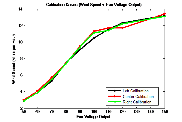
The above graph shows a calibration curve for the wind tunnel before testing. The graph displays a pretty even distribution of wind speed throughout the tunnel. Even though the speed may vary with certain fan voltages the speeds are basically the same throughout.
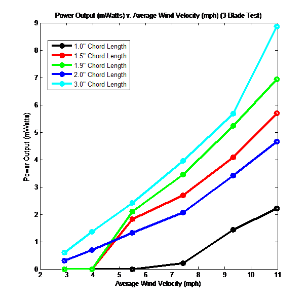
The above graph shows the power output versus the average wind velocity for the tests involving three blades on the wind turbine. In this portion of the experiment all of the shapes are the same, oval, but the difference between them is the various chord lengths. According to the graph the blades with the three inch chord length had the highest power output versus the other blades, while the one inch blade length had the least amount of power output. Even though it was expected that the three-inch blades would have the highest output and the one-inch blades would have the lowest output, the blades with the 1.5 inch, 1.9 inch, and 2.0 inch chord lengths show a different trend. Our group believed that the power output would be highest with the highest chord length, but the data shows that the 1.9 inch blade chord length had the second highest result, then the 1.5 inch chord length, and finally the 2.0 inch chord length. This may be a result because this test did not reach the maximum power output, so no conclusion can be based on this data, until this maximum is reached.
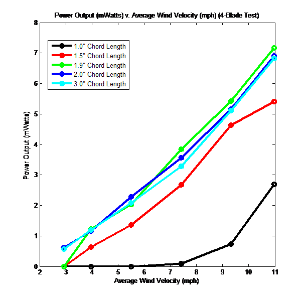
From the above graph, we can say that once again the 1.0” chord length performs the worst. The 3.0” chord length blade was again at or near the best output; however the 1.9” and 2.0” chord length blades performed extremely close to that of the 3.0” chord length blade. We did notice that the 1.9” chord length blade did not perform very well at very low wind speeds as you can see the curve for that blade is well below that of the 3.0” chord length blade. Out of the three(1.9”, 3.0”, 2.0”) chord length blades at high wind speeds, we cannot determine which will perform the best considering that they are so close in terms of output and the power curves haven’t come near to reaching their maximum output. Had we been able to test the blades up to their actual output maximum, we may see a large difference.
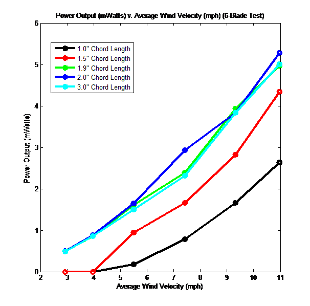
As is seen from the above curve the 1.0” and 1.5” chord length blades had trouble picking up the lower wind velocity due to the lack of sufficient surface needed to do so. The 1.9” and the 3.0” chord length blades have shown to be extremely similar in our test using six blades. We believe that it is too early to arrive at any conclusion for why this may be so due to the inability of these blades to reach a maximum. The 2.0” chord length blade has proven in this case to be the most effective but again it is too early to say that it will remain the most effective even at higher wind velocities.
2 Comments
sgrace posted on December 10, 2012 at 1:52 pm
Please show the geometry of the blades.
I don’t understand how there are 3 different graphs if the only thing that changed was the chord length and the results for the varying chordlength are shown on the curve. Please explain the conditions to which the different curves refer.
dehrenp posted on December 10, 2012 at 4:09 pm
The titles of the graphs showed how each of the graphs differed. Each graph (with the various amounts of power curves) represents a different amount of blades being tested (i.e. the first graph corresponds to 3-blades being tested for each chord length, the second graph corresponds to 4-blades being tested for each chord length, and the third graph corresponds to 6-blades being tested for each chord length). The introduction should have included that the number of blades was another variable that was changing throughout the experiment. Finally, our blade geometry was all ovals (with no change i shape). This was mentioned in the introduction. Do we also need to post a picture of an oval?