This post is a short summary of a Machine Learning project I completed in 2022. This was my very first project in machine learning! It has been peer-reviewed and published in the open-access Frontiers Journal: https://doi.org/10.3389/fspas.2022.858990. You can find the GitHub repository of the trained model here.
Outline:
- Quick Intro to the Space Physics Problem
- Problem Description & Motivation
- Data & Dataset Preparation
- Deep Learning Model Inputs, Outputs and Architecture
- Results: Model Performance
- Results: Classifying Events
- Results: Application on POES Data
- Challenges & Solutions
- Summary
1. Quick Intro to the Space Physics Problem
Energetic (>500 keV) electrons populate the Earth’s Van Allen Belts (also known as the radiation belts) and can fall into the atmosphere after interacting with electromagnetic waves in the near-Earth environment. Energetic electron precipitation (EEP) can also occur when the terrestrial magnetic field is stretched away from Earth (phenomenon also called current sheet scattering, CSS). These two mechanisms (wave vs CSS) produce a different type of precipitation into Earth’s atmosphere. Waves drive spatially localized high-energy (>~700 keV) precipitation, while field line stretching drives precipitation at several energies (from low to high) and with energy dependence (i.e., low-energy electrons precipitate at higher latitudes than high-energy electrons). Characterizing the properties of EEP is fundamental to understand a) the dynamics of the near-Earth environment and b) how much energy this phenomenon deposits in our atmosphere. Electron precipitation is one outcome of the perturbations of the terrestrial magnetic field, mostly driven by the Sun’s activity. EEP also has several repercussions on our atmosphere as it can alter its chemistry and possibly contribute to ozone destruction, together with impacting the reliability of communication systems.
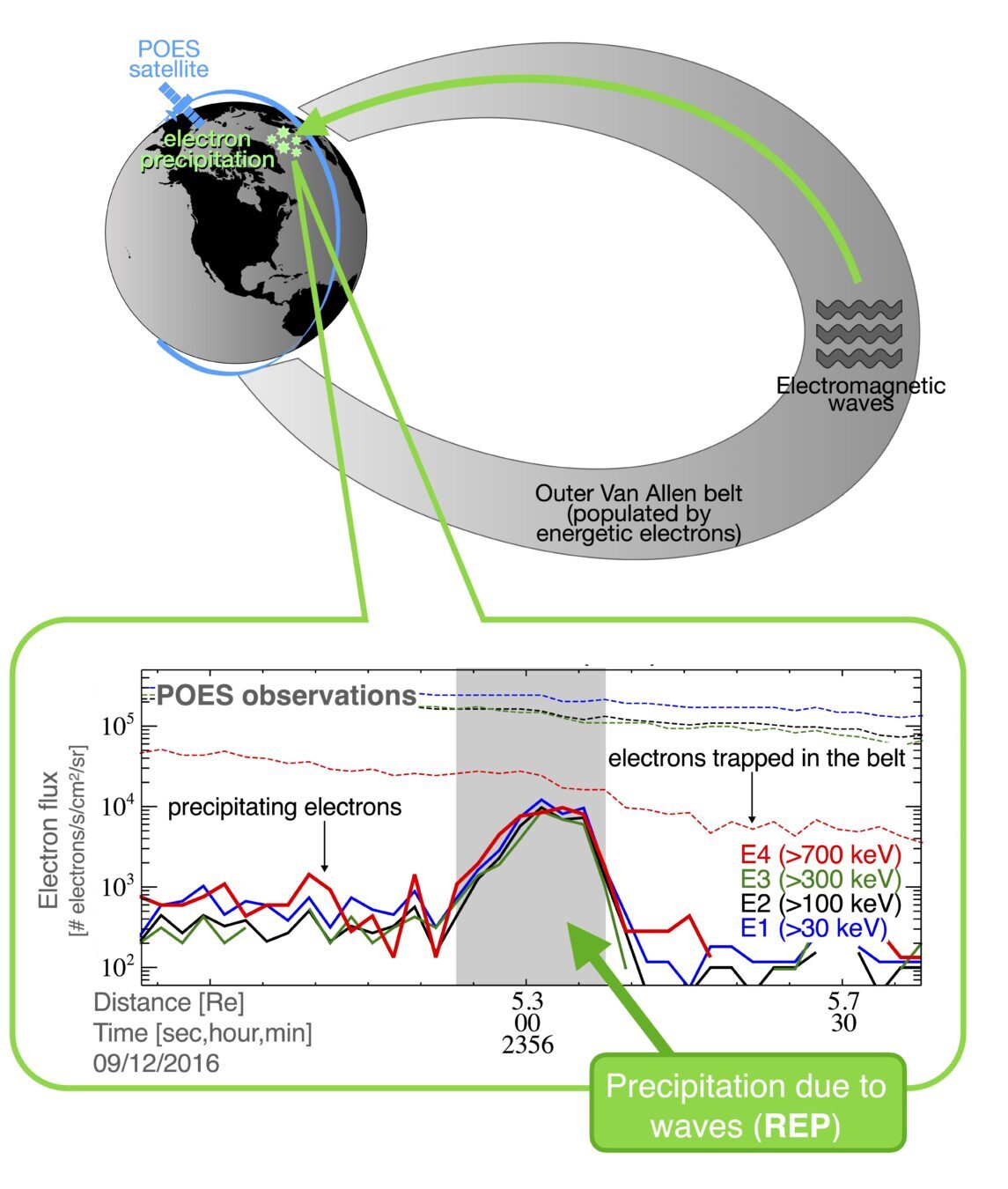
Fig 1. Cartoon of wave-driven EEP (REP) and POES observations at low-Earth-orbit.
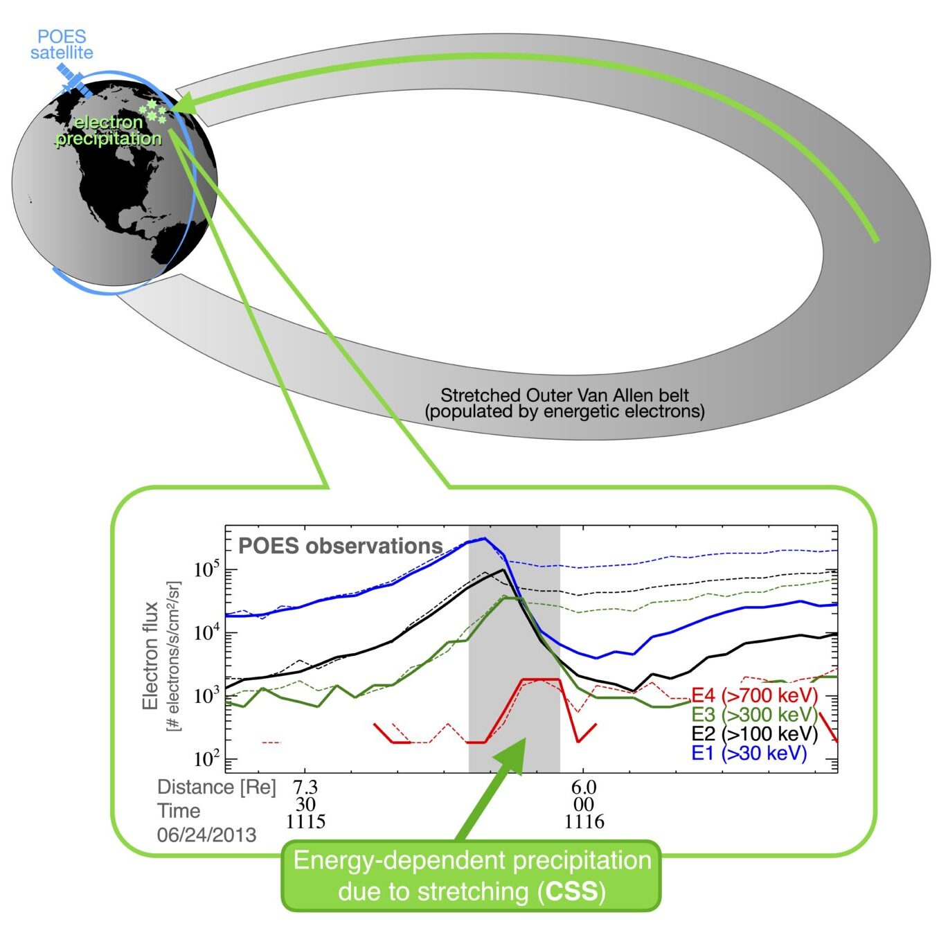
Fig 2. Cartoon of stretching-driven precipitation (CSS) and POES observations at low-Earth-orbit.
2. Problem Description & Motivation
EEP occurs frequently, but its observation depends on the spatial coverage of low-Earth-orbit (LEO) satellites. Algorithms have been proposed to identify electron precipitation, however, they rely on arbitrary flux thresholds, do not account for the precipitation efficiency, and might include only strong precipitation. Most importantly, algorithms require a high level of complexity if we aim to distinguish between the driving mechanism (waves vs CSS). Here, I show you a supervised deep learning multi-class classification technique that automatically a) identifies and b) classifies electron precipitation by its associated driver. My main objective is to automatically categorize events by drivers with an acceptable (though not perfect) performance. I anticipated that a certain degree of post-processing and/or visual scrutiny of the model results would be necessary before they could be utilized for scientific research.
3. Data & Dataset Preparation
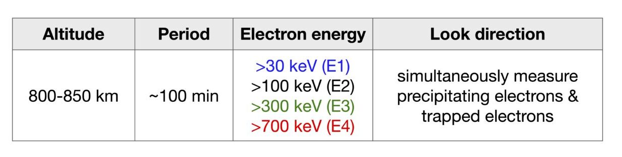
I use 2-second electron flux measured by the NOAA POES and EUMETSAT MetOp satellites (public data), which have extensive coverage in space (latitude/longitude) and time (available since at least 2012 ). More specs are in the following table.
As for any supervised task, we need a ground truth of the EEP events, separated by category (waves vs CSS). I manually collected 230 wave-EEP (called REP) and 174 stretching-EEP (CSS) events from 2012 to 2020 – all looking very similar to those in Fig 1 and Fig 2. The datapoints nearby the events are counted as “no-event” (class 0). REP are class 1, CSS are class 2. Clearly, we cannot use entire POES orbit since the EEP events are so short-lived (~10s seconds) – the model would only learn the “no-event” category (Fig 9). To overcome this, we consider a window of 50 datapoints for each event and place the event at its center (Fig 3). We assign the class of 1 or 2 to the datapoints in the event boundaries and leave to 0 the rest of the datapoints. We make sure that the class 1 and 2 events have clear boundaries and truly belong to one class or the other, and we also guarantee that the 0 class data points indeed do not show precipitation. The class (also called label/target) is one-hot encoded; in other words, 3 binary digits indicate the class: 1-0-0 is class 0, 0-1-0 is class 1, and 0-0-1 is class 2. We randomly stack events and also augment the dataset by mirroring each event by its center point, for a total of 460 REP and 348 CSS (~40,400 data points). Data gaps and null fluxes are replaced with 0.01 (100) s−1cm−2sr−1 for the precipitating (trapped) telescope measurements.
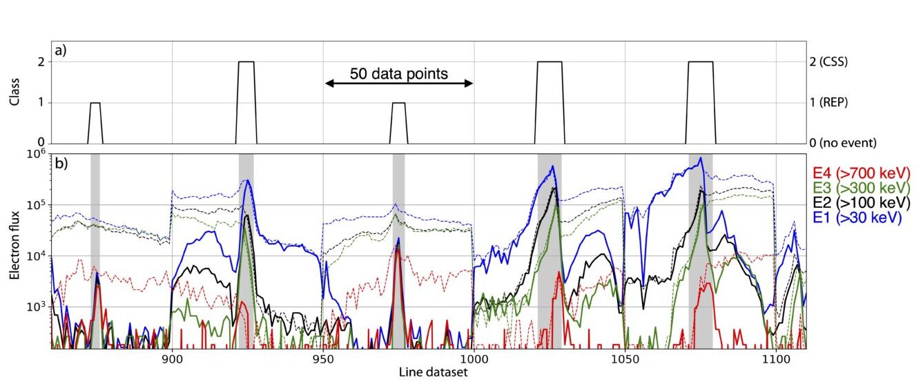
Fig 3. Portion of the train dataset. Top: class. Bottom: electron flux for precipitating (solid line) and trapped (dashed line) energy channel (color-coded in the legend).
4. Deep Learning Model Inputs, Outputs and Architecture
As a matter of fact, we are dealing with a time-series classification, so I chose to use the LSTM architecture. The time variable is not explicit in the dataset, however, it is intrinsically represented by the profile of the precipitation (isolated for REP and with energy-dependency for CSS) as the satellite orbits through the precipitation region. The next section will demonstrate LSTM is suitable for this specific project and I also found it outperforms other multi-layer perceptron (MLP) architectures.
The LSTM structure requires inputs to be a tensor (basically, a matrix of multiple dimensions). I select 7-point-long snapshots of the dataset and assign to each snapshot one class. The class for each snapshot is the most common class in the 7-point-long class snapshot (inspired by this blog post). That is, if the snapshot is partly including a CSS event (Fig 4), then the most common class is the CSS class (2). Snapshots have stride of 1 data point. The entire input dataset is fed into the model as a tensor that spans the entire dataset (with blocks of 7 data points, advancing with stride 1). The model ingests one snapshot at a time and associates with (thus tries to learn) its most common class. The data inputs are the 8 electron fluxes at the 4 energy channels (E1, E2, E3, E4) for both the trapped and precipitating electrons. The model output is the one-hot encoded class.
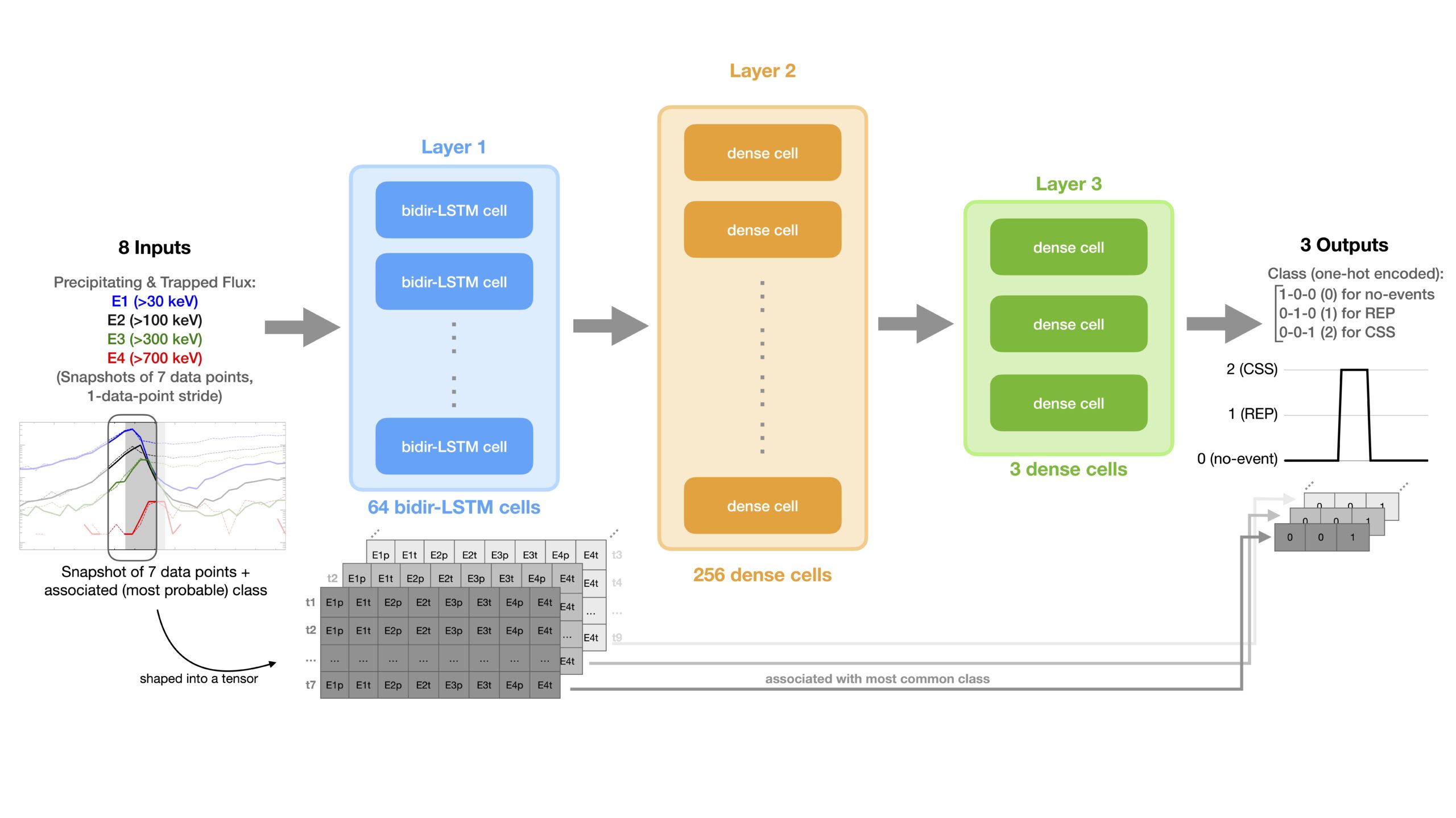
Fig 4. Deep Learning Model Architecture, with inputs and outputs.
After a few trials with different configurations, I adopted an architecture of 64 bidirectional LSTM cells (layer 1; ReLu activation function), followed by 256 dense (fully connected; ReLu activation function) cells (layer 2), with a final output layer of 3 dense cells (layer 3; softmax activation function) as shown in Fig 4. This results in ~70,000 free parameters. Dropouts at 0.5 rates are between the layer 1 and 2 and layer 2 and 3, and help in avoiding overfitting, though I found they are not critical to achieve a good performance.
5. Results: Model Performance
The metrics used is that of classification problems, with particular attention to the F1 score (weighted average of the precision and recall), the AUC (area under the ROC (Receiver Operating Characteristic) recall vs false-positive-rate curve) and the AUPRC (area under the precision vs. recall curve). During training, we use early stopping (with patience of 10 epochs) on the AUC calculated for the validation dataset. I also performed a k-fold cross validation with k = 10, to make sure the model does not perform exceptionally well for a specific subset of the dataset and poorly on other subsets. In simple terms, the dataset of 40,400 points is split into 10 sections: 9 are used for training and 1 is used for testing. 15% of the training set (i.e., the 9 sections) are used for validation. The single section used for testing changes every k iteration, thus we will have 10 models with a specific performance. The final model performance is the average of the performances of the 10 models. The final model is trained using the entire dataset, reserving 15% for validation purposes. The model has a performance of F1∼0.948, AUC∼0.995, and AUPRC∼0.990 (across all 3 classes). The confusion matrix (averaged across all k-folds) is shown in Fig 5. The performance scores are very high because the model does a great job at predicting the 0-class events (as this is the most numerous class). The F1 per class is: 0.97 for class 0, 0.83 for class 1 (REP), and 0.87 for class 2 (CSS).
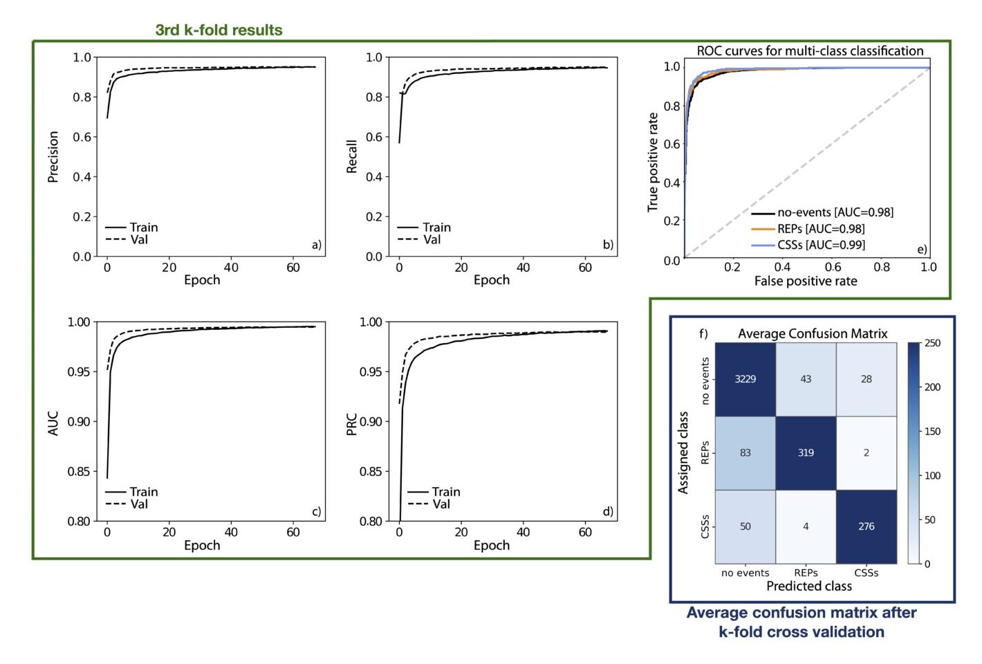
Fig 5. Green: Results from the 3rd k-fold. Blue: confusion matrix after cross validation.
6. Results: Classifying events
Fig 6 below shows the performance of the model on a portion of the test dataset: the model correctly identifies no-events, REP and CSS. Obviously, the model results are not perfect and indeed the width of the events is not exactly as that manually set in the test dataset and it is not precisely centered at the event. You can see a small shift of the label to the left, which we attribute to the fact each class is assigned as the most common label of the 7-point-long snapshot. To clarify, the initial snapshot undergoes classification using the most likely label among the first seven data points. As the sliding window advances with a stride of 1, each label becomes linked to the subsequent 7 data points, causing some shift. This is easily fixable by adding a systematic delay to the output label. Additionally, given the intrinsic probabilistic outcome of the ML model, the 0-1-2 labels indicate the probable location of the no-event, REP or CSS rather than the exact location of these categories.
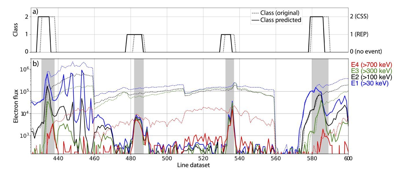
Fig 6. Portion of the test dataset with a) assigned class (dashed) and predicted class (solid line); b) electron flux used as input.
7. Results: Application on Realistic Data
The previous section shows the application of the model on the test dataset which, by definition, is structured exactly as the training dataset. In practice, we should apply the model to the realistic data observed by POES during its orbit. We note that the model does a good job in identifying the EEP events and also in assigning them to the correct categories. Some post-processing is needed to improve the model outputs, but the results are acceptable enough already and I did not believe continuing to fine-tune the model or the dataset was worth pursuing for my ultimate goal.
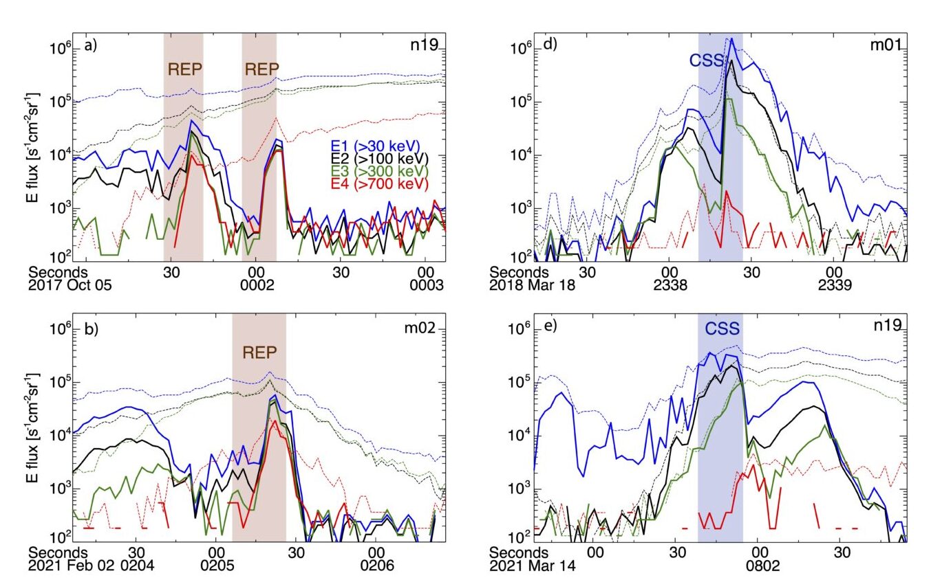
Fig 7. Examples of the model applied to four days of POES data.
Obviously, the model is not perfect and some false positives are still possible. So, in order to build a dataset of reliable REP and CSS events, a visual inspection of the results is still preferred, especially to use the events for scientific research.
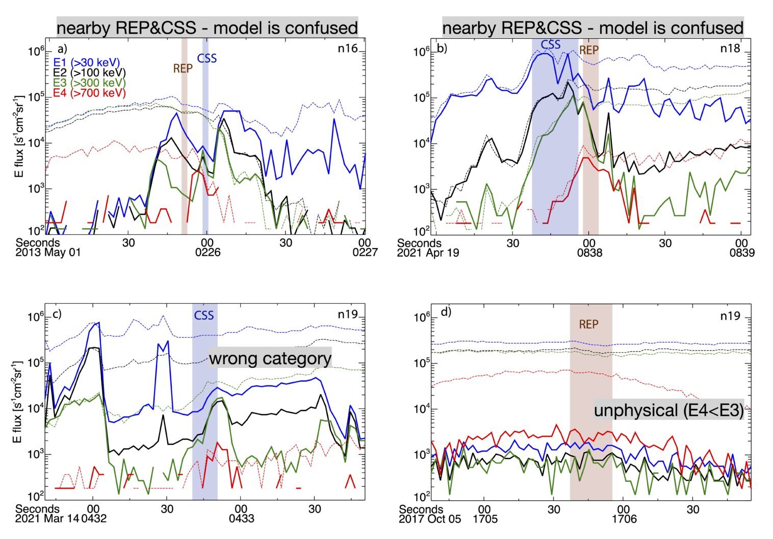
Fig 8. Examples of false positives identified by the model.
8. Challenges & Solutions
Model only learns the no-event class: if we feed into the model the entire orbit of POES (~100min of data) with class 1 or 2 for REP or CSS, the model only learns the 0 class because REP and CSS occur infrequently over 1 POES orbit (~once at max). Solution: crop the POES data around the EEP event (e.g., with a 50-point-long window) and assign label 1 or 2 to the event boundary and 0 elsewhere.
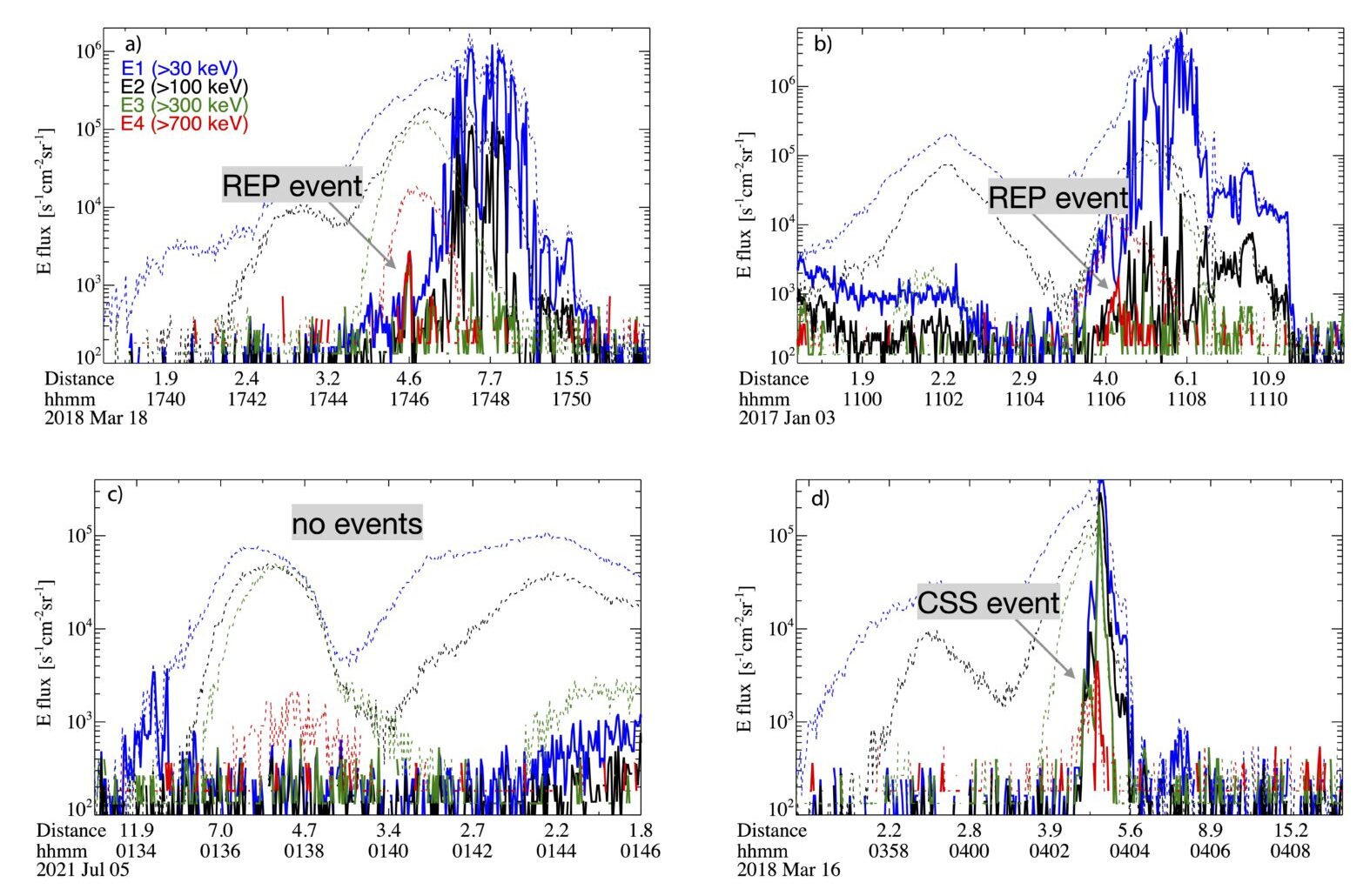
Fig 9. Examples of a quarter orbit of POES. POES crosses the outer belt in a matter of ~10min. REP and CSS are only lasting ~10s seconds.
Imbalanced dataset: only ∼20% of the data points are labeled with 1 or 2 (this dataset is still imbalanced with respect to the 0 class). Solution: the REP and CSS classes are approximately balanced (∼10% data points are REPs and ∼8% data points are CSSs) and the model is able to identify correctly no-events, REPs and CSSs. I avoided applying other known solutions (augmentation, weighted sampling, etc.) to overcome the imbalanced nature of the dataset because a) the model results were acceptable for my goal and b) I preferred maintaining a readable dataset and avoid disrupting the time-series sequence by performing weighted sampling or relying on other solutions.
Model wasn’t identifying the entire extent of the events: my initial dataset labeled as 1 or 2 only a few points (typically the center points with high E4 flux) as “events” an the model was not able to identify many events at all. Solution: the labels have to be nearly perfect and cover the exact extent of the precipitation events. I realized the model performance improved significantly once the labels were defining the event boundaries more appropriately. This is not surprising as this is a supervised ML task and the ground truth (training dataset) should indeed be as perfect as possible such that the model can learn from it.
Model performance is good, but the results are not perfect (false positives): given the F1 scores I reported above, once would assume this model is nearly perfect, however, false positives and incorrectly categorized events are still possible given the imbalanced dataset. Solution: in my case, I was happy with a working ML model that provided good-enough results that I could improve further by visual inspection, so I stopped in attempting to further fine-tune the model. My ultimate goal is to obtain a reliable dataset of REP and CSS events on a large amount of years in order to conduct scientific research. Therefore, visual inspection to guarantee that indeed these events are correctly identified and categorized is needed no matter how good the model is. Obviously, if this model should be used without human visual inspection (e.g., as a tool onboard of satellites), one should improve the model to limit the number of false positives.
9. Summary
Algorithms exist that identify energetic electron precipitation (EEP) events from POES data, however they rely significantly on arbitrary flux thresholds and do not categorize the events by driver (waves or CSS). My objective is to build a ML tool that automatically identifies events and also categorizes them into REP (wave-drive EEP) and CSS (stretching-driven EEP). This is a time-series multi-class classification which I achieve using an LSTM architecture. The trained model has F1~0.948 and acceptably provides the REP and CSS events. Post-processing and visual inspection of the results are needed to limit the number of false positives. My ultimate goal is to obtain lists of REP and CSS events that span the entire lifetime of the POES satellite data (decades) and perform scientific statistical analysis and research on the datasets.
Some resources I used:
TensorFlow Tutorials (time-series forecasting, classification, imbalanced data)
Towards Data Science “Multi-Class Metrics Made Simple, Part I: Precision and Recall” blog post
Note: this post is a short summary of my original peer-reviewed paper, which you can find here https://doi.org/10.3389/fspas.2022.858990. You can find the GitHub repository of the trained model here.