Category Archives: EC 581

ACA versus GOP plans side-by-side

This article from the LA Times by columnist Noam Levey links an update on earlier postings online that does a side-by-side comparison of ACA versus the GOP’s replacement AHCA plan. That posting provides the best concise overview I have seen of the latest GOP AHCA proposal. It will take 10 minutes to review/read. Randy

Here is the comparison

http://www.latimes.com/projects/la-na-pol-obamacare-repeal/


Here is the new article, which features specific effects.

http://www.latimes.com/la-na-pol-obamacare-repeal-chaos-20170625-story.html


From: Levey, Noam [mailto:Noam.Levey@latimes.com]
Sent: Sunday, June 25, 2017 9:44 PM
To: Levey, Noam
Subject: ICYMI: New article on the disruptive impact of the Senate repeal bill

Good day,

In case you missed it, I wanted to share my latest piece examining the potentially devastating impact of the recently released Senate legislation to roll back the Affordable Care Act.

The Republican architects of the bill, like their House counterparts, hail their legislation as a remedy for ills caused by the current law. But across the country, in physicians’ offices and medical centers, in state capitols and corporate offices, there is widespread fear the unprecedented cuts in the GOP bills would create even larger problems in the U.S. healthcare system, threatening to not only strip health coverage from millions, but also upend insurance markets, cripple state budgets and drive medical clinics and hospitals to the breaking point. As Tom Tom Priselac, chief executive of Cedars Sinai Health System in Los Angeles, told me: “These reductions are going to wreak havoc.”

Here is the link: http://www.latimes.com/la-na-pol-obamacare-repeal-chaos-20170625-story.html

I hope you find the piece interesting. Thank you, as always, for reading. All best,

-N

Noam N. Levey

National healthcare reporter

Los Angeles Times Washington Bureau

Tel: 202-824-8317

Cell: 202-247-0811

noam.levey@latimes.com

twitter: @NoamLevey

Economist article about end of life planning

One of my students today just sent me this link to an article in this week’s Economist about end-of-life planning.

How to have a better death

http://www.economist.com/news/leaders/21721371-death-inevitable-bad-death-not-how-have-better-death

It led me to also view its link about conversations about serious illness by one of my favorite authors.

“Serious Illness Conversation Guide” drawn up by Atul Gawande

I also found these slides targeting providers informative as well.

Using the Serious Illness Conversation Guide - HealthInsight

I found it informative that CMS (Medicare) created two new Advance Care Planning (ACP) codes. It will be interesting to see how often they are used.

Two new codes created in 2015, allowed for payment by Medicare in 2016.

  • 99497 ACP 30 minutes $85.99
  • 99498 ACP additional 30 minutes $74.88

CPT describes eligible services as being performed by a physician or “other qualified health professional” which means a physician, NP or PA.

We could save a lot of money and improve happiness and quality of life if more doctors, nurses, families and patients talked about these issues.


Obamacare reality: It is working

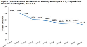
At a time in the US when all of the Republicans presidential candidates are declaring Obamacare a failure which needs to be undone, it is worth noting the REALITY that it is succeeding in its primary purpose of covering more American with health insurance. It does not mandate insurance coverage, but the subsidies and tax penalties for not having insurance are motivating more people to get insurance. 20 million more people now have health insurance than did before. (Click on graphs for a clearer image.)

 20 Million Gained Health Insurance From Obamacare, President Says
The Huffington Post

Uninsured rate Gallop-HealthwaysEven though cost containment was not its primary goal, Obamacare is also reducing, not increasing, costs of health care.
Since many people don’t trust the government, here are some private sector slides.
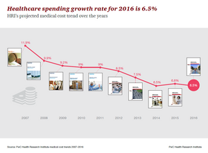
PriceWaterhouseCoopers, an actuary firm not known for being political, forecasts that health expenditure
cost growth in 2016 will continue to slow down.

http://www.pwc.com/us/en/health-industries/behind-the-numbers/assets/pwc-hri-medical-cost-trend-chart-pack-2016.pdf

Here are my two favorite slides from their chart pack. Note the changes since 2010.

pwc trends gdpand nhe

My view is that the above figure is misleading, since the decline in rates of growth did not start in 1961, but still the slow growth since 2010 is clearly evident.


spending growth rate PWC 2016

Obamacare is working. We just don’t have enough leaders and media telling us this.


Note: I sent this blog to my BUHealth email list.

Let me know if you would like to be added as a BUHealthFriends subscriber by emailing ellisrp at bu.edu

Ellis SAS tips for experienced SAS users

If you are a beginning SAS programmer, then the following may not be particularly helpful, but the books suggested in the middle may be. BU students can obtain a free license for SAS to install on their own computer if it is required for a course or research project. Both will require an email from an adviser. SAS is also available on various computers in the economics department computer labs.

I also created a Ellis SAS tips for new SAS programmers.

I do a lot of SAS programming on large datasets, and thought it would be productive to share some of my programming tips on SAS in one place. Large data is defined to be a dataset so large that it cannot be stored in the available memory. (My largest data file to date is 1.7 terabytes.)

Suggestions and corrections welcome!

Use SAS macro language whenever possible;

It is so much easier to work with short strings than long lists, especially with repeated models and datasteps;

%let rhs = Age Sex HCC001-HCC394;


Design your programs for efficient reading and writing of files, and minimize temporary datasets.

SAS programs on large data are generally constrained by IO (input output, reading from your hard drives), not by CPU (actual calculations) or memory (storage that disappears once your sas program ends). I have found that some computers with high speed CPU and multiple cores are slower than simpler computers because they are not optimized for speedy hard drives. Large memory really helps, but for really huge files it can almost almost be exceeded, and then your hard drive speeds will really matter. Even reading in and writing out files the hard drive speeds will be your limiting factor.

This implication of this is that you should do variable creation steps in as few datastep steps as possible, and minimize sorts, since reading and saving datasets will take a lot of time. This requires a real change in thinking from STATA, which is designed for changing one variable at a time on a rectangular file. Recall that STATA can do this efficiently since it usually starts by bringing the full dataset into memory before doing any changes. SAS does not do this, one of its strengths.

Learning to use DATA steps and PROC SQL is the central advantage of an experienced SAS programmer. Invest, and you will save time waiting for your programs to run.

Clean up your main hard drive if at all possible.

Otherwise you risk SAS crashing when your hard drive gets full. If it does, cancel the job and be sure to delete the temporary SAS datasets that may have been created before you crashed. The SAS default for storing temporary files is something like

C:\Users\"your_user_name".AD\AppData\Local\Temp\SAS Temporary Files

Unless you have SAS currently open, you can safely delete all of the files stored in that directory. Ideally, there should be none since SAS deletes them when it closes normally. It is the abnormal endings of SAS that cause temporary files to be saved. Delete them, since they can be large!

Change the default hard drive for temporary files and sorting

If you have a large internal secondary hard drive with lots of space, then change the SAS settings so that it uses temp space on that drive for all work files and sorting operations.

To change this default location to a different internal hard drive, find your sasv9.cfg file which is in a location like

"C:\Program Files\SASHome\x86\SASFoundation\9.3\nls\en"

"C:\Program Files\SASHome2-94\SASFoundation\9.4\nls\en"

Find the line in the config firl that starts -WORK and change it to your own location for the temporary files (mine are on drive j and k) such as:

-WORK "k:\data\temp\SAS Temporary Files"

-UTILLOC "j:\data\temp\SAS Temporary Files"

The first one is where SAS stores its temporary work files such as WORK.ONE where you define the ONE such as by DATA ONE;

The second line is where SAS stores its own files such as when sorting a file or when saving residuals.

There is a reason to have the WORK and UTIL files on different drives, so that it is in generally reading in from one drive and writing out to a different one, rather than reading in and writing out on the same drive. Try to avoid the latter. Do some test on your own computer to see how much time you can save by switching from one drive to another instead of only using one drive.

Use only internal hard drives for routine programming

Very large files may require storage or back up on external hard drives, but these are incredibly slow. External drives are three to ten times slower than an internal hard drive. Try to minimize their use for actual project work. Instead, buy more internal drives if possible. You can purchase additional internal hard drives with 2T of space for under $100. You save that much in time the first day!

Always try to write large datasets to a different disk drive than you read them in from.

Do some tests copying large files from c: to c: and from C: to F: You may not notice any difference until the file sizes get truly huge, greater than your memory size.

Consider using binary compression to save space and time if you have a lot of binary variables.

By default, SAS stores datasets in  a fixed rectangular dataset that leaves lots of empty space when you use integers instead of real numbers. Although I have been a long time fan of using OPTIONS COMPRESS=YES to save space and run time (but not CPU time) I only recently discovered that

OPTIONS COMPRESS=BINARY;

is even better for integers and binary flags when they outnumber real numbers. For some large datasets with lots of zero one dummies it has reduced my file size by as much as 97%! Standard variables are stored as 8 bytes, which have 8*256=2048 bits. In principle you could store 2000 binary flags in the space of one real number. Try saving some files on different compression and see if your run times and storage space improve. Note: compression INCREASES files size for real numbers! It seems that compression saves space when binary flags outnumber real numbers or integers;

Try various permutations on the following on you computer with your actual data to see what saves time and space;

data real;           retain x1-x100 1234567.89101112; do i = 1 to 100000; output; end;run; proc means; run;

data dummies; retain d1-d100 1;                                do i = 1 to 100000; output; end; proc means; run;

*try various datasteps with this, using the same or different drives. Bump up the obs to see how times change.


Create a macro file where you store macros that you want to have available anytime you need them. Do the same with your formats;

options nosource;
%include "c://data/projectname/macrofiles";
%include "c://data/projectname/allformats";
options source;

Be aware of which SAS procs create large, intermediate files

Some but not all procs create huge temporary datasets.

Consider: PROC REG, and PROC GLM generates all of the results in one pass through the data unless you have an OUTPUT statement. Then they create large,uncompressed, temporary files that can be a multiple of your original file sizes. PROC SURVEYREG and MIXED create large intermediate files even without an output statement. Plan accordingly.

Consider using OUTEST=BETA to more efficiently create residuals together with PROC SCORE.

Compare two ways of making residuals;

*make test dataset with ten million obs, but trivial model;

data test;
do i = 1 to 10000000;
retain junk1-junk100 12345;  * it is carrying along all these extra variables that slows SAS down;
x = rannor(234567);
y = x+rannor(12345);
output;
end;

Run;    * 30.2 seconds);
*Straightforward way; Times on my computer shown following each step;
proc reg data = test;
y: model y = x;
output out=resid (keep=resid) residual=resid;
run;  *25 seconds;
proc means data = resid;
run;  *.3 seconds;

*total of the above two steps is 25.6 seconds;

proc reg data = test outest=beta ;
resid: model y = x;
run;                     *3.9 seconds;
proc print data = beta;
run;  *take a look at beta that is created;
proc score data=test score=beta type=parms
out=resid (keep=resid) residual;
var x;
run;       *6 seconds!;
proc means data = resid;
run;  .3 seconds;

*total from the second method is 10.3 seconds versus 25.6 on the direct approach PLUS no temporary files needed to be created that may crash the system.

If the model statement in both regressions is

y: model y = x junk1-junk100; *note that all of the junk has coefficients of zero, but SAS does not this going in;

then the two times are

Direct approach:    1:25.84
Scoring approach:  1:12.46 on regression plus 9.01 seconds on score = 1:21.47 which is a smaller savings

On very large files the time savings are even greater because of the reduced IO gains; SAS is still able to do this without writing onto the hard drive in this "small" sample on my computer. But the real savings is on temporary storage space.

Use a bell!

My latest addition to my macro list is the following bell macro, which makes sounds.

Use %bell; at the end of your SAS program that you run batch and you may notice when the program has finished running.

%macro bell;
*plays the trumpet call, useful to put at end of batch program to know when the batch file has ended;
*Randy Ellis and Wenjia Zhu November 18 2014;
data _null_;
call sound(392.00,70); *first argument is frequency, second is duration;
call sound(523.25,70);
call sound(659.25,70);
call sound(783.99,140);
call sound(659.25,70);
call sound(783.99,350);
run;
%mend;
%bell;

Purchase essential SAS programming guides.

I gave up on purchasing the paper copy of SAS manuals, because they take up more than two feet of shelf space, and are still not complete or up to date. I find the SAS help menus useful but clunky. I recommend the following if you are going to do serious SAS programming. Buy them used on Amazon or whatever. I would get an older edition, and it will cost less than $10 each. Really.

The Little SAS Book: A Primer, Fifth Edition (or an earlier one)

Nov 7, 2012

by Lora Delwiche and Susan Slaughter

Beginners introduction to SAS. Probably the best single book to buy when learning SAS.
 

Professional SAS Programmer's Pocket Reference Paperback

By Rick Aster

http://www.amazon.com/Professional-SAS-Programmers-Pocket-Reference/dp/189195718X

Wonderful, concise summary of all of the main SAS commands, although you will have to already know SAS to find it useful. I use it to look up specific functions, macro commands, and optoins on various procs because it is faster than using the help menus. But I am old style...

Professional SAS Programming Shortcuts: Over 1,000 ways to improve your SAS programs Paperback

By Rick Aster

http://www.amazon.com/Professional-SAS-Programming-Shortcuts-programs/dp/1891957198/ref=sr_1_1?s=books&ie=UTF8&qid=1417616508&sr=1-1&keywords=professional+sas+programming+shortcuts

I don't use this as much as the above, but if I had time, and were learning SAS instead of trying to rediscover things I already know, I would read through this carefully.

Get in the habit of deleting most intermediate permanent files

Delete files if either

1. You won't need them again or

2. You can easily recreate them again.  *this latter point is usually true;

Beginner programmers tend to save too many intermediate files. Usually it is easier to rerun the entire program instead of saving the intermediate files. Give your final file of interest a name like MASTER or FULL_DATA then keep modifying it by adding variables instead of names like SORTED, STANDARDIZED,RESIDUAL,FITTED.

Consider a macro that helps make it easy to delete files.

%macro delete(library=work, data=temp, nolist=);

proc datasets library=&library &nolist;
delete &data;
run;
%mend;

*sample macro calls

%delete (data=temp);   *for temporary, work files you can also list multiple files names but these disappear anyway at the end of your run;

%delete (library =out, data = one two three) ; *for two node files in directory in;

%delete (library=out, data =one, nolist=nolist);   *Gets rid of list in output;


Ellis SAS tips for New SAS programmers

There is also a posting on Ellis SAS tips for Experienced SAS programmers

It focuses on issues when using large datasets.


Randy’s SAS hints for New SAS programmers, updated Feb 21, 2015

  1. ALWAYS

    begin and intermix your programs with internal documentation. (Note how I combined six forms of emphasis in ALWAYS: color, larger font, caps, bold, italics, underline.) Normally I recommend only one, but documenting your programs is really important. (Using only one form of emphasis is also important, just not really important.)

A simple example to start your program in SAS is

******************
* Program = test1, Randy Ellis, first version: March 8, 2013 – test program on sas features
***************;

Any comment starting with an asterisk and ending in a semicolon is ignored;


    1. Most common errors/causes of wasted time while programming in SAS.

a. Forgetting semicolons at the end of a line

b. Omitting a RUN statement, and then waiting for the program to run.

c. Unbalanced single or double quotes.

d. Unintentionally commenting out more code than you intend to.

e. Foolishly running a long program on a large dataset that has not first been tested on a tiny one.

f. Trying to print out a large dataset which will overflow memory or hard drive space.

g. Creating an infinite loop in a datastep; Here is one silly one. Usually they can be much harder to identify.

data infinite_loop;
x=1;
nevertrue=0;
do while x=1;
if nevertrue =1 then x=0;
end;
run;

h. There are many other common errors and causes of wasted time. I am sure you will find your own


  1. With big datasets, 99 % of the time it pays to use the following system OPTIONS:


options compress =yes nocenter;

or

options compress =binary nocenter;

binary compression works particularly well with many binary dummy variables and sometimes is spectacular in saving 95%+ on storage space and hence speed.


/* mostly use */
options nocenter /* SAS sometimes spends many seconds figuring out how to center large print outs of
data or results. */
ps=9999               /* avoid unneeded headers and page breaks that split up long tables in output */
ls=200;                /* some procs like PROC MEANS give less output if a narrow line size is used */
 

*other key options to consider;

Options obs = max   /* or obs=100, Max= no limit on maximum number of obs processed */
Nodate nonumber /* useful if you don’t want SAS to embed headers at top of each page in listing */
Macrogen     /* show the SAS code generated after running the Macros. */
Mprint   /* show how macro code and macro variables resolve */
nosource /* suppress source code from long log */
nonotes   /* be careful, but can be used to suppress notes from log for long macro loops */

;                       *remember to always end with a semicolon!;


  1. Use these three key procedures regularly

Proc contents data=test; run; /* shows a summary of the file similar to Stata’s DESCRIBE */
Proc means data = test (obs=100000); run; /* set a max obs if you don’t want this to take too long */
Proc print data = test (obs=10); run;


I recommend you create and use regularly a macro that does all three easily:

%macro cmp(data=test);
Proc Contents data=&data; Proc means data = &data (obs=1000); Proc print data = &data (obs=10); run;
%end;

Then do all three (contents, means, print ten obs) with just

%cmp(data = mydata);


  1. Understand temporary versus permanent files;

Data one;   creates a work.one temporary dataset that disappears when SAS terminates;

Data out.one; creates a permanent dataset in the out directory that remains even if SAS terminates;


Define libraries (or directories):

Libname out “c:/data/marketscan/output”;
Libname in “c:/data/marketscan/MSdata”;


Output or data can be written into external files:

Filename textdata “c:/data/marketscan/textdata.txt”;


  1. Run tests on small samples to develop programs and then Toogle between tiny and large samples when debugged.

A simple way is

Options obs =10;
*options obs = max; *only use this when you are sure your programs run.
 

OR, some procedures and data steps using End= dataset option do not work well on partial samples. For those I often toggle between two different input libraries. Create a subset image of all of your data in a separate directory and then toggle using the libname commands;


*Libname in ‘c:/data/projectdata/fulldata’;
Libname in ‘c:/data/projectdata/testsample’;


Time spent creating a test data set is time well spent.

You could even write a macro to make it easy. (I leave it as an exercise!)


  1. Use arrays abundantly. You can use different array names to reference the same set of variables. This is very convenient;


%let rhs=x1 x2 y1 y2 count more;
Data _null_;
Array X {100} X001-X100; *usual form;
Array y {100} ;                     * creates y1-y100;
Array xmat {10,10} X001-X100; *matrix notation allows two dimensional indexes;
Array XandY {*} X001-X100 y1-y100 index ; *useful when you don’t know the count of variables in advance;
Array allvar &rhs. ;     *implicit arrays can use implicit indexes;
 

*see various ways of initializing the array elements to zero;

Do i = 1 to 100; x{i} = 0; end;
 

Do i = 1 to dim(XandY); XandY{i} = 0; end;


Do over allvar; allvar = 0; end;   *sometimes this is very convenient;


Do i=1 to 100 while (y(i) = . );
y{i} = 0;   *do while and do until are sometimes useful;
end;


run;

  1. For some purposes naming variables in arrays using leading zeros improves sort order of variables

Use:
Array x {100} X001-X100;
not
Array x {100} X1-X100;

With the second, the alphabetically sorted variables are x1,x10,x100, x11, x12,..,x19, x2,x20 , etc.


  1. Learn Set versus Merge command (Update is for rare, specialized use)


Data three;   *information on the same person combined into a single record;
Merge ONE TWO;
BY IDNO;
Run;


  1. Learn key dataset options like

Obs=
Keep=
Drop=
In=
Firstobs=
Rename=(oldname=newname)
End=


  1. Keep files being sorted “skinny” by using drop or keep statements

Proc sort data = IN.BIG(keep=IDNO STATE COUNTY FROMDATE) out=out.bigsorted;
BY STATE COUNTY IDNO FROMDATE;
Run;

Also consider NODUP and NODUPKEY options to sort while dropping duplicate records, on all or on BY variables, respectively.


  1. Take advantage of BY group processing

Use FIRST.var and LAST.var abundantly.


USE special variables
_N_ = current observation counter
_ALL_ set of all variables such as Put _all_. Or when used with PROC CONTENTS, set of all datasets.


Also valuable is

PROC CONTENTS data = in._all_; run;


  1. Use lots of comments


* this is a standard SAS comment that ends with a semicolon;


/*   a PL1 style comment can comment out multiple lines including ordinary SAS comments;

* Like this; */


%macro junk; Macros can even comment out other macros or other pl1 style comments;

/*such as this; */ * O Boy!; %macro ignoreme;   mend; *very powerful;


%mend; * end macro junk;


  1. Use meaningful file names!

Data ONE TWO THREE can be useful.


  1. Put internal documentation about what the program does, who did it and when.
  2. Learn basic macro language; See SAS program demo for examples. Know the difference between executable and declarative statements used in DATA step


17. EXECUTABLE COMMANDS USED IN DATA STEP (Actually DO something, once for every record)


Y=y+x (assignment. In STATA you would use GEN y=x or REPLACE Y=X)
 
Do I = 1 to 10;
End; (always paired with DO, can be nested nearly unlimited deepness)


INFile in ‘c:/data/MSDATA/claimsdata.txt’;               define where input statements read from;
File out ‘c:/data/MSDATA/mergeddata.txt’;             define where put statements write to;


Goto johnny;      * always avoid. Use do groups instead;


IF a=b THEN y=0 ;
ELSE y=x; * be careful when multiple if statements;
CALL subroutine(); (Subroutines are OK, Macros are better)


INPUT   X ; (read in one line of X as text data from INFILE)
PUT   x y= / z date.; (Write out results to current LOG or FILE file)


MERGE IN.A IN.B ;
BY IDNO;         *   Match up with BY variable IDNO as you simultaneously read in A&B;

Both files must already be sorted by IDNO.

SET A B;                                           * read in order, first all of A, and then all of B;

UPDATE   A B; *replace variables with new values from B only if non missing in B;


OUTPUT out.A;      *Write out one obs to out.A SAS dataset;
OUTPUT;                *Writes out one obs of every output file being created;

DELETE;   * do not output this record, and return to the top of the datastep;

STOP;                               * ends the current SAS datastep;


18. Assignment commands for DATA Step are

only done once at the start of the data step


DATA ONE TWO IN.THREE;

*This would create three data sets, named ONE TWO and IN.THREE

Only the third one will be kept once SAS terminates.;

Array x {10} x01-x10;
ATTRIB x length =16 Abc length=$8;
RETAIN COUNT 0;
BY state county IDNO;
Also consider  
BY DESCENDING IDNO; or BY IDNO UNSORTED; if grouped but not sorted by IDNO;
DROP i;   * do not keep i in final data set, although it can still be used while the data step is running
KEEP IDNO AGE SEX; *this will drop all variables from output file except these three;
FORMAT x date.;   *permanently link the format DATE. To the variable link;

INFORMAT ABC $4.;

LABEL AGE2010 = “Age on December 31 2010”;
LENGTH x 8; *must be assigned the first time you reference the variable;
RENAME AGE = AGE2010; After this point you must use the newname (AGE2010);
OPTIONS NOBS=100; One of many options. Note done only once.


19. Key Systems language commands

LIBNAME to define libraries
FILENAME to define specific files, such as for text data to input or output text

TITLE THIS TITLE WILL APPEAR ON ALL OUTPUT IN LISTING until a new title line is given;

%INCLUDE

%LET year=2011;

%LET ABC = “Randy Ellis”;


20. Major procs you will want to master

DATA step !!!!! Counts as a procedure;

PROC CONTENTS

PROC PRINT

PROC MEANS

PROC SORT

PROC FREQ                      frequencies

PROC SUMMARY      (Can be done using MEANS, but easier)

PROC CORR (Can be done using Means or Summary)

PROC REG       OLS or GLS

PROC GLM   General Linear Models with automatically created fixed effects

PROC FORMAT /INFORMAT

PROC UNIVARIATE

PROC GENMOD nonlinear models

PROG SURVEYREG clustered errors

None of the above will execute unless a new PROC is started OR you include a RUN; statement.

21. Formats are very powerful. Here is an example from the MarketScan data. One use is to simply recode variables so that richer labels are possible.


Another use is to look up or merge on other information in large files.


Proc format;
value $region
1=’1-Northeast Region           ‘
2=’2-North Central Region       ‘
3=’3-South Region               ‘
4=’4-West Region               ‘
5=’5-Unknown Region             ‘
;


value $sex

1=‘1-Male           ‘
2=‘2-Female         ‘
other=‘ Missing/Unknown’

;


*Three different uses of formats;

Data one ;
sex=’1’;
region=1;
Label sex = ‘patient sex =1 if male’;
label region = census region;
run;

Proc print data = one;

Run;


data two;
set one;
Format sex $sex.; * permanently assigns sex format to this variable and stores format with the dataset;
Run;

Proc print data = two;
Run;

Proc contents data = two;
Run;

*be careful if the format is very long!;


Data three;
Set one;
Charsex=put(sex,$sex.);
Run;

*maps sex into the label, and saves a new variable as the text strings. Be careful can be very long;

Proc print data =three;
Run;


Proc print data = one;
Format sex $sex.;
*this is almost always the best way to use formats: Only on your results of procs, not saved as part of the datasets;
Run;


If you are trying to learn SAS on your own, then I recommend you buy:

The Little SAS Book: A Primer, Fifth Edition (or an earlier one)

Nov 7, 2012

by Lora Delwiche and Susan Slaughter

Beginners introduction to SAS. Probably the best single book to buy when learning SAS.

Recommended book on US health care system

I highly recommend this book as a useful summary of the US Health Care System. I have made it required reading (as a reference) for my classes at BU.

The Health Care Handbook: A Clear and Concise Guide to the United States Health Care System, 2nd Edition Paperback – November 15, 2014

by Elisabeth Askin (Author), Nathan Moore (Author)


Paper:  $15.99

http://www.amazon.com/gp/product/0692244735

Electronic: $8.99

http://www.amazon.com/Health-Care-Handbook-Concise-United-ebook/dp/B00PWQ93M8/


Explaining these two graphs should merit a Nobel prize

Reposting from The Incidental Economist Blog

What happened to US life expectancy?

Posted: 07 Jan 2014 03:00 AM PST

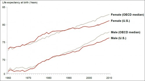
Here’s another chart from the JAMA study “The Anatomy of Health Care in the United States”:

life expectancy at birth

Why did the US fall behind the OECD median in the mid-1980s for men and the early 1990s for women? Note, the answer need not point to the health system. But, if it does, it’s not the first chart to show things going awry with it around that time. Before I quote the authors’ answer, here’s a related chart from the paper:

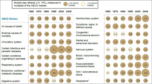
ypll

The chart shows years of potential life lost in the US as a multiple of the OECD median and over time. Values greater than 1 are bad (for the US). There are plenty of those. A value of exactly 1 would mean the US is at the OECD median. Below one would indicate we’re doing better. There’s not many of those.

It’d be somewhat comforting if the US at least showed improvement over time. But, by and large, it does not. For many conditions, you can see the US pulling away from the OECD countries beginning in/around 1980 or 1990, as was the case for life expectancy shown above. Why?

The authors’ answer:

Possible causes of this departure from international norms were highlighted in a 2013 Institute of Medicine report and have been ascribed to many factors, only some of which are attributed to medical care financing or delivery. These include differences in cultural norms that affect healthy behaviors (gun ownership, unprotected sex, drug use, seat belts), obesity, and risk of trauma. Others are directly or indirectly attributable to differences in care, such as delays in treatment due to lack of insurance and fragmentation of care between different physicians and hospitals. Some have also suggested that unfavorable US performance is explained by higher risk of iatrogenic disease, drug toxicity, hospital-acquired infection, and a cultural preference to “do more,” with a bias toward new technology, for which risks are understated and benefits are unknown. However, the breadth and consistency of the US underperformance across disease categories suggests that the United States pays a penalty for its extreme fragmentation, financial incentives that favor procedures over comprehensive longitudinal care, and absence of organizational strategy at the individual system level. [Link added.]

This is deeply unsatisfying, though it may be the best explanation available. Nevertheless, the sentence in bold is purely speculative. One must admit that it is plausible that fragmentation, incentives for procedures, and lack of organizational strategy could play a role in poor health outcomes in the US — they certainly don’t help — but the authors have also ticked off other factors. Which, if any, dominate? It’s completely unclear.

Apart from the explanation or lack thereof, I also wonder how much welfare has been lost relative to the counterfactual that the US kept pace with the OECD in life expectancy and health spending. It’s got to be enormous unless there are offsetting gains in areas of life other than longevity and physical well-being. For example, if lifestyle is a major contributing factor, perhaps doing and eating what we want (to the extent we’re making choices) is more valuable than lower mortality and morbidity. (I doubt it, but that’s my speculation/opinion.)

(I’ve raised some questions in this post. Feel free to email me with answers, if you have any.)

@afrakt

Two great reposts from TIE/JAMA

This repost from The Incidental Economist (TIE) is one of the best summaries of US Health Care I have seen. I also appended the Uwe posting at the bottom.

(The JAMA Authors are Hamilton Moses III, MD; David H. M. Matheson, MBA, JD; E. Ray Dorsey, MD, MBA; Benjamin P. George, MPH; David Sadoff, BA; Satoshi Yoshimura, PhD

The JAMA Article, which has an abundance of tables, references and graphs, will be on my MA and Ph.D. reading lists.

Anyone interested in keeping up with current US health policy from an economists point of view should subscribe to TIE, although it can be distracting, frustrating, and time consuming.

Randy

Study:The Anatomy of Health Care in the United States

Posted: 13 Nov 2013 03:55 AM PST

From JAMA. I reformatted the abstract, and broke it up into paragraphs to make it easier to read:

Health care in the United States includes a vast array of complex interrelationships among those who receive, provide, and finance care. In this article, publicly available data were used to identify trends in health care, principally from 1980 to 2011, in the source and use of funds (“economic anatomy”), the people receiving and organizations providing care, and the resulting value created and health outcomes.

In 2011, US health care employed 15.7% of the workforce, with expenditures of $2.7 trillion, doubling since 1980 as a percentage of US gross domestic product (GDP) to 17.9%. Yearly growth has decreased since 1970, especially since 2002, but, at 3% per year, exceeds any other industry and GDP overall.

Government funding increased from 31.1% in 1980 to 42.3% in 2011. Despite the increases in resources devoted to health care, multiple health metrics, including life expectancy at birth and survival with many diseases, shows the United States trailing peer nations. The findings from this analysis contradict several common assumptions. Since 2000,

  1. price (especially of hospital charges [+4.2%/y], professional services [3.6%/y], drugs and devices [+4.0%/y], and administrative costs [+5.6%/y]), not demand for services or aging of the population, produced 91% of cost increases;
  2. personal out-of-pocket spending on insurance premiums and co-payments have declined from 23% to 11%; and
  3. chronic illnesses account for 84% of costs overall among the entire population, not only of the elderly.

Three factors have produced the most change:

  1. consolidation, with fewer general hospitals and more single-specialty hospitals and physician groups, producing financial concentration in health systems, insurers, pharmacies, and benefit managers;
  2. information technology, in which investment has occurred but value is elusive; and
  3. the patient as consumer, whereby influence is sought outside traditional channels, using social media, informal networks, new public sources of information, and self-management software.

These forces create tension among patient aims for choice, personal care, and attention; physician aims for professionalism and autonomy; and public and private payer aims for aggregate economic value across large populations. Measurements of cost and outcome (applied to groups) are supplanting individuals’ preferences. Clinicians increasingly are expected to substitute social and economic goals for the needs of a single patient. These contradictory forces are difficult to reconcile, creating risk of growing instability and political tensions. A national conversation, guided by the best data and information, aimed at explicit understanding of choices, tradeoffs, and expectations, using broader definitions of health and value, is needed.

My frustration? That anyone treats any of this as news. At some point we need to stop diagnosing the problem and start doing something about it.

The whole thing is worth a read. But none of it will be news for regular visitors to TIE. Why isn’t everyone reading this blog already?!?!?!

@aaronecarroll

Quote: Uwe (Need I say more?)

Posted: 13 Nov 2013 04:00 AM PST

[T]he often advanced idea that American patients should have “more skin in the game” through higher cost sharing, inducing them to shop around for cost-effective health care, so far has been about as sensible as blindfolding shoppers entering a department store in the hope that inside they can and will then shop smartly for the merchandise they seek. So far the application of this idea in practice has been as silly as it has been cruel. [...]

In their almost united opposition to government, US physicians and health care organizations have always paid lip service to the virtue of market, possibly without fully understanding what market actually means outside a safe fortress that keeps prices and quality of services opaque from potential buyers. Reference pricing for health care coupled with full transparency of those prices is one manifestation of raw market forces at work.

-Uwe Reinhardt, The Journal of the American Medical Association. I thank Karan Chhabra for the prod.

@afrakt

AHRF/ARF 2012-13 data is available free

AHRF=Area Health Resource File (Formerly ARF)

2012-2013 ARHF can now be downloaded at no cost.

The 2012-2013 ARF data files and documentation can now be downloaded. Click the link below to learn how to download ARF documentation and data.

http://arf.hrsa.gov/

“The Area Health Resources Files (AHRF)—a family of health data resource
products—draw from an extensive county-level database assembled annually from
over 50 sources. The AHRF products include county and state ASCII files, an MS Access
database, an AHRF Mapping Tool and Health Resources Comparison Tools (HRCT). These
products are made available at no cost by HRSA/BHPR/NCHWA to inform health resources
planning, analysis and decision making..”

"The new AHRF Mapping Tool enables users to compare the availability of healthcare providers as well as environmental factors impacting health at the county and state levels."

2007-2020 MarketScan Data at Boston University

Boston University is now in its third year of licensing use to the MarketScan Commercial Claims and Encounters databases. This data is available for free to Boston University faculty, staff, and students for unfunded research, but researchers are required to request funding for any externally funded research projects. Interested researchers should contact Randy Ellis, who is data manager for the data.

The Truvan Analytics MarketScan Commercial Claims Databases provide individual-level clinical utilization, expenditures, and enrollment across inpatient, outpatient, prescription drug, and carve-out services from a selection of large employers and health plans. The MarketScan Databases link paid claims and encounter data to detailed patient information across sites and types of providers, and over time. The annual medical databases include private sector health data from approximately 100 payers. Historically, more than 500 million claim records are available in the MarketScan Databases. These data represent the medical experience of insured employees and their dependents for active employees, early retirees, COBRA continues and Medicare-eligible retirees with employer-provided Medicare Supplemental plans.

While the information about the individuals is rather limited (age, gender, employment status, industry, MSA, enrollment information, plan type), the information about their utilization of medical care is incredibly detailed. Some of the most useful variables are: Out-of-pocket payment (sub-divided into deductible, coinsurance, and copayments) and total payment by service rather than by admission, detailed diagnosis and procedure codes, service codes, precise dates of visits and admissions, provider-type, and facility information. The data also included detailed information on prescription drug claims including information for identifying the specific (down to the dose) drug purchased, the amount purchased, and the date of refills.

This vast amount of information allows researchers to construct general variables such as the financial risk of an enrollee (in terms of an age-gender and diagnosis-based risk score), an enrollee’s annual out-of-pocket expenses, geographic variation in spending, geographic variation in the use of a particular procedure or drug down to the state and MSA-level (State and county and 3-digit zip code-level in 2007-2010 data). It also allows researchers to construct more detailed individual-level variables such as cancer diagnosis and subsequent chemotherapy use, ER admission and subsequent readmissions, individual preferences for brand vs. generic pharmaceuticals, etc.

There are separate tables for enrollee information (individual-level), outpatient claims (service-level), inpatient services (service-level), inpatient admissions (admission-level; aggregated version of inpatient services), prescription drug claims (prescription/refill-level), and facility information (facility-level). All of these tables can be linked using a unique enrollee ID. The unique enrollee IDs are constant across years, allowing researchers to follow individuals over time as long as they remain insured by the same payer.

The information in these tables comes directly from the payers (employers and insurance plans). Truven Analytics then cleans and verifies the data from each payer, de-identifies the data it, and combines it to form the final dataset. Because the data come from the payers, and the payers are paying Truven Analytics to provide them with accurate information and analysis about the claims, the incentives are aligned to provide accurate data.

The data includes an electronic copy of the Red Book list of all pharmaceuticals marketed in the US, along with information about each of the 350,000+ NDC (National Drug Code) values. Significant detail about the data is available in the accompanying data description and data quality appendices.

The versions we have use a six month claims “runout”, which is to say that claims for 2011 services are accepted through the June 30, 2012.

The following table includes additional year-specific information about the data files:

Year Number of Individuals Size of all files Geographic Detail
2007 35,305,924 203 GB MSA, 3-digit zip code & county
2008 41,275,020 251 GB MSA, 3-digit zip code & county
2009 39,970,145 263 GB MSA, 3-digit zip code & county
2010 45,239,752 281 GB MSA, 3-digit zip code & county
2011 52,194,324 321 GB MSA and state ONLY
Total 213,985,165 1.319 TB


Commonwealth Fund Report on Health Care Cost Control

The Commonwealth Fund has just come out with a new report outlining a strategy for containing health care costs in the US. It seems rather optimistic to me. Here is the opening two paragraphs and link.

Confronting Costs: Stabilizing U.S. Health Spending While Moving Toward a High Performance Health Care System, Authored by The Commonwealth Fund Commission on a High Performance Health System
January 10, 2013

Michael Chernew (Harvard) is the only economist on the Commission, which is mostly MDs and MBAs.

"Overview

The Commonwealth Fund Commission on a High Performance Health System, to hold increases in national health expenditures to no more than long-term economic growth, recommends a set of synergistic provider payment reforms, consumer incentives, and systemwide reforms to confront costs while improving health system performance. This approach could slow spending by a cumulative $2 trillion by 2023—if begun now with public and private payers acting in concert. Payment reforms would: provide incentives to innovate and participate in accountable care systems; strengthen primary care and patient-centered teams; and spread reforms across Medicare, Medicaid, and private insurers. With better consumer information and incentives to choose wisely and lower provider administrative costs, incentives would be further aligned to improve population health at more affordable cost. Savings could be substantial for families, businesses, and government at all levels and would more than offset the costs of repealing scheduled Medicare cuts in physician fees." from The Commonwealth Fund Report

The heart of their analysis is in the technical report by Actuarial Research Corp.

Jim Mays, Dan Waldo, Rebecca Socarras, and Monica Brenner "Technical Report: Modeling the Impact of Health Care Payment, Financing, and System Reforms" Actuarial Research Corporation, January 10, 2013

The areas they simulate are revealed in the table of content headings. Nice recent references.

Introduction .................................................................................................................................................. 1
I. Improved Provider Payment ................................................................................................................. 4
II. Primary Care: Medical Homes ............................................................................................................... 7
III. High-Cost Care Management Teams .................................................................................................. 13
IV. Bundled Payments .............................................................................................................................. 16
V. Modified Payment Policy for Medicare Advantage ............................................................................ 22
VI. Medicare Essential Benefits Plan ........................................................................................................ 26
VII. Private Insurance: Tightened Medical Loss Ratio Rules ...................................................................... 30
VIII. Reduced Administrative Costs and Regulatory Burden ...................................................................... 32
IX. Combined Estimates ........................................................................................................................... 35
X. Setting Spending Targets .................................................................................................................... 37
Appendix A. Creating the "Current Policy" Baseline ................................................................................... 40


US Cardiovascular Diseases Rates are Improving But…

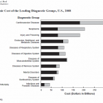
I browsed to the following overview of US research on Heart, Lung, and Blood diseases in the US. This report documents the dramatic improvements in cardiovascular health in the US, which they estimate costs the US about $300 billion or about $1000 per American in 2008 (Direct of treatment and indirect costs from premature mortality).  This makes the US look good, until they compare this trend to trends in other countries, which are almost all better, and have also had large decreases in mortality from 2000 to 2008. We currently spend $3 billion per year on research on Heart, Lung and Blood diseases ($10 per American per year). Below are three figures all from this one report.

http://www.nhlbi.nih.gov/about/factbook/FactBook2011.pdf


HCC risk adjustment formulas for ACA Exchanges

HHS announced the new risk adjustment formulas proposed for the ACA Health Insurance Exchanges on December 7, 2012.
Here is the citation and direct link.
Department of Health and Human Services. HHS Benefit and Payment Parameters for 2014, and Medical Loss Ratio. 2012 [Dec 7 2012]. Available from: http://www.gpo.gov/fdsys/pkg/FR-2012-12-07/pdf/2012-29184.pdf
Focus only on the first 33 pages for teh Risk adjustment system.
Summary:
This proposed regulations provides details on the risk adjustment formula that is proposed for the Federal and STate Health insurance exchanges. At its heart is an HCC model similar to the Medicare 100 condition HCC model. Innovations are that it has separate models for four metal levels (bronze, silver, gold, platinum), it uses a concurrent rather than prospective framework, it has separate models for infants, children and adults. It was estimated at RTI using Truven Health Analytics 2010 MarketScan® data, which we also have licensed at Boston University for research use. The rules are a painful 373 pages long. Focus on pages 1-33 for an overview of the RA approach.
Other NPRM (=Notice of Proposed Rule Making) for regulations of the ACA are the following.
EHB/AV (Essential Health Benefits/Actuarial Value) NPRM:
Summary: http://www.healthcare.gov/news/factsheets/2012/11/ehb11202012a.html
Citation: US National Archives and Records Administration. 2012. Code of Federal Regulations. Title 45. Patient Protection and Affordable Care Act; Standards Related to Essential Health Benefits, Actuarial Value, and Accreditation; Proposed Rule. [Available at: http://www.regulations.gov/#!documentDetail;D=CMS-2012-0142-0001]

Discussion: The rule discusses accreditation of health plans in a federally-facilitated or state-federal partnership exchange. States that plans offered inside and outside of the exchange must offer a core package of benefits including the following: Ambulatory patient services, emergency services, hospitalization, maternity and newborn care, mental health and substance use disorder services, prescription drugs, rehabilitative services, lab services, preventive and wellness services and chronic disease management, and pediatric services.

The rule also specifies options for each state's "benchmark" plan. Plans must offer coverage greater than or equal to that offered by the benchmark plan.

The rule also specifies that HHS will provide an AV calculator to help issuers determine health plan ACs. The calculator uses a nationally representative sample. Starting in 2015, HHS will accept state-specific datasets to use with the calculator. The rule proposes a 2% AV window around the AV specified by for each metal group.

Market Reform NPRM:
Rule: http://www.regulations.gov/#!documentDetail;D=CMS-2012-0141-0001
 

Citation: US National Archives and Records Administration. 2012. Code of Federal Regulations. Title 45. Patient Protection and Affordable Care Act; Health Insurance Market Rules; Rate Review; Proposed Rule. [Available at: http://www.regulations.gov/#!documentDetail;D=CMS-2012-0141-0001]

Discussion: This rule focuses on reforms to the health insurance market. It includes guaranteed issue, premium regulation (rate bands, rate restrictions), single statewide risk pool, etc. The rule also proposes regulation changes to streamline data collection.

MPFS (Medicare Physician Fee Schedule) Rule:
Citation: US National Archives and Records Administration. 2012. Code of Federal Regulations. Title 42. Medicare Program; Revisions to Payment Policies Under the Physician Fee Schedule, DME Face-to-Face Encounters, Elimination of the Requirement for Termination of Non- Random Prepayment Complex Medical Review and Other Revisions to Part B for CY 2013. [Available at: http://www.gpo.gov/fdsys/pkg/FR-2012-11-16/pdf/2012-26900.pdf]
More rules and regulations are presented here.
I thank without implicating Tim Layton (BU RA extraordinaire) for organizing this information for me.

Lisa Iezzoni’s new book on Risk Adjustment****

I just received and have scanned through Lisa Iezzoni's fourth book (as editor and major contributor) entitled

Risk Adjustment for Measuring Health Care Outcomes (Fourth Edition), Lisa I Iezzoni (ed) (2013)

Even though Lisa is a physician, not an economist or statistician, this book provides an excellent overview of risk adjustment (population-based), and severity or case mix adjustment (episode or event based), and includes discussion of available datasets, model comparisons, propensity score matching, lists of information potentially useful, clinical classification, variables  clinical, social and statistical issues. Contributions on statistical methodology by Michael Swartz and Arlene Ash, as well as separate chapters on mental health, long term care, managing healthcare organizations, and provider profiling are excellent. Its main weakness is in not capturing international developments at all, not discussing the commercial market for risk adjustment models, and not covering most nonlinear and econometric (as distinct from statistical) issues well. Still, it should be required reading for anyone planning to do work in this area.

I have put it on my list of all time favorite books, but acknowledge that only a limited subset of people will be interested in it.


Comprehensive Primary Care Initiative, by CMS, Overview

CMS posted in late August an interesting site that provides lots of information about the seven demonstrations going on for Comprehensive Primary Care Payment.

http://innovations.cms.gov/initiatives/Comprehensive-Primary-Care-Initiative/index.html
Each site includes a list of participating PCPs. with specific clinic names, zip codes and addresses. Could be interesting to examine how severe a selection problem there is.

Five Questions for Health Economists

My presidential address to the American Society of Health Economists is now available to download and scheduled for publication in the International Journal of Health Care Finance and Economics. Here is the link.

Five questions for health economists

Randall P. Ellis

Online First™, 3 September 2012

Here is the direct link to the pdf file.

http://www.springerlink.com/content/7m2668027362x52r/fulltext.pdf


Ash and Ellis “Risk-adjusted Payment and Performance Assessment for Primary Care” is out

After working in the area for the past three years, I am happy to report that the paper below is finally out in  Medical Care.

Risk-adjusted Payment and Performance Assessment for Primary Care

Ash, Arlene S. PhD; Ellis, Randall P. PhD

The full version is currently posted as printed ahead of print, although the actual date of the publication is not yet known. You will need a OVID or a Lippincott Williams & Wilkins subscription to have access to the full paper. you can see if your university has access by visiting the site above. There is also a rich appendix with further results and tables.

Abstract
Background: Many wish to change incentives for primary care practices through bundled population-based payments and substantial performance feedback and bonus payments. Recognizing patient differences in costs and outcomes is crucial, but customized risk adjustment for such purposes is underdeveloped.

Research Design: Using MarketScan's claims-based data on 17.4 million commercially insured lives, we modeled bundled payment to support expected primary care activity levels (PCAL) and 9 patient outcomes for performance assessment. We evaluated models using 457,000 people assigned to 436 primary care physician panels, and among 13,000 people in a distinct multipayer medical home implementation with commercially insured, Medicare, and Medicaid patients.

Methods: Each outcome is separately predicted from age, sex, and diagnoses. We define the PCAL outcome as a subset of all costs that proxies the bundled payment needed for comprehensive primary care. Other expected outcomes are used to establish targets against which actual performance can be fairly judged. We evaluate model performance using R2's at patient and practice levels, and within policy-relevant subgroups.

Results: The PCAL model explains 67% of variation in its outcome, performing well across diverse patient ages, payers, plan types, and provider specialties; it explains 72% of practice-level variation. In 9 performance measures, the outcome-specific models explain 17%-86% of variation at the practice level, often substantially outperforming a generic score like the one used for full capitation payments in Medicare: for example, with grouped R2's of 47% versus 5% for predicting "prescriptions for antibiotics of concern."

Conclusions: Existing data can support the risk-adjusted bundled payment calculations and performance assessments needed to encourage desired transformations in primary care.

(C) 2012 Lippincott Williams & Wilkins, Inc.

It is currently only available as a publication ahead of print, 2012 Apr 19. [Epub ahead of print]

http://journals.lww.com/lww-medicalcare/Abstract/publishahead/Risk_adjusted_Payment_and_Performance_Assessment.99429.aspx

Risk-adjusted Payment and Performance Assessment for Primary Care.
Ash AS, Ellis RP.

2012 Handbook of Health Economics, on ScienceDirect

2012 Handbook of Health Economics (Pauly, McGuire and Barros) is free on-line. Here is the link to the pdf files.

Excellent literature reviews and new insights. I purchased the hard cover version, but this is wonderfully accessible.

http://www.sciencedirect.com/science/handbooks/15740064

Many research universities, including BU have access to ScienceDirect.

It is unusual for Elsevier to post its new material for free access in this way.

Enjoy.

US Physician office visits declined 17% from 2009-2011

Being insured is no guarantee unemployed will seek care

Research suggests they may be unable to cover co-pays and deductibles, or fear they cannot afford the expenses that result.

By Victoria Stagg Elliott, amednews staff. Posted Feb. 7, 2012.

Unemployed people who have private health insurance are less likely to put off care because of cost than those without insurance or on public plans. But they are much more likely than the employed to stay away from the doctor's office.

"Even if you have insurance, you typically have to pay 20% or more of the price, and when you become unemployed, you become more cautious about spending money," said Randall Ellis, PhD, professor of economics at Boston University and president of the American Society of Health Economists. "You put off preventive visits, and if you have the flu, you choose not to go in for treatment."

About 29.3% of the unemployed had private insurance, according to a data brief issued Jan. 24 by the Centers for Disease Control and Prevention's National Center for Health Statistics analyzing adults 18-64 who participated in the National Health Interview Survey for 2009-2010 (www.cdc.gov/nchs/data/databriefs/db83.htm).

Full article is here.

http://www.ama-assn.org/amednews/2012/02/06/bisd0207.htm

Puzzling fact is that outpatient office visits declined by 17%:

"Outpatient office visits declined 17% among patients with private insurance -- from 156 million in the second quarter of 2009 to 129 million in the second quarter of 2011."

(Ibid)

Yet  total private insurance spending on physicians remained almost unchanged.

2009 2010 Change
Total $408.3 billion $415.8 billion 1.8%
Private insurance $209.0 billion $209.4 billion 0.2%

Source: National Health Expenditure Data, Centers for Medicare & Medicaid Services Office of the Actuary, January (www.cms.gov/nationalhealthexpenddata/01_overview.asp)

Also see: http://www.ama-assn.org/amednews/2012/01/23/gvl10123.htm

Could be worth exploring...

ARF 2009-10 is available free

ARF=Area Resource File

2009-2010 ARF Can Now Be Downloaded at No Cost.

The 2009-2010 ARF data files and documentation can now be downloaded. Click the link below to learn how to download ARF documentation and data.

http://arf.hrsa.gov/purchase.htm

"The basic county-specific Area Resource File (ARF) is the nucleus of the overall ARF System. It is a database containing more than 6,000 variables for each of the nation's counties. ARF contains information on health facilities, health professions, measures of resource scarcity, health status, economic activity, health training programs, and socioeconomic and environmental characteristics. In addition, the basic file contains geographic codes and descriptors which enable it to be linked to many other files and to aggregate counties into various geographic groupings."

"You may also choose to search the ARF to see what data variables are available in the current file."

The table of contents below gives a sense of the county level information included.


I.       DATA ELEMENT DESCRIPTIONS AND REFERENCES. 1
A.  CODES AND CLASSIFICATIONS. 1
A-1)        Header for ARF. 1
A-2)        State and County Codes. 1
A-3)        Census County Group Codes. 7
A-4)        County Typology Codes. 7
A-5)        Metropolitan/Micropolitan and Combined Statistical Areas. 10
A-6)        Rural/Urban Continuum Codes. 11
A-7)        Urban Influence Codes. 13
A-8)        BEA Economic Area Codes and Names and Component Economic 14                          Area Codes and Names.
A-9)        Federal Region Code and Census Region and Division Codes and Names. 14
A-10)     Veterans Administration Codes. 16
A-11)     Contiguous Counties. 17
A-12)     Health Service Area Codes. 18
A-13)     Area Health Education Center (AHEC) Codes and Names. 18
A-14)     HPSA Codes. 19
A-15)     SSA Beneficiary State and County Codes. 21
B.   HEALTH PROFESSIONS. 22
B-1)        Physicians. 22
B-2)        Dentists and Dental Hygienists. 31
B-3)        Optometrists. 36
B-4)        Pharmacists. 37
B-5)        Podiatrists. 38
B-6)        Veterinarians. 39
B-7)        Nurses. 40
B-8)        Physician Assistants. 43
B-9)        Chiropractors. 45
B-10)      Occupational Therapists. 46
B-11)      Physical Therapists. 46
B-12)      Psychology and Social Work Teachers. 47
B-13)      Psychologists. 47
B-14)      Sociologists. 48
B-15)      Social Workers. 48
B-16)     Audiologists   49
B-17)     Speech Language Pathologists  49
B-18)      Healthcare Practitioner Professionals. 50
B-19)      Decennial Census Occupation Data. 50
C.  HEALTH FACILITIES. 53
C-1)        Hospital Type. 54
C-2)        Hospital Services (or Facilities) 57
C-3)        Hospital Employment 57
C-4)        Nursing and Other Health Facilities. 58
C-5)        Health Maintenance Organizations. 60
C-6)        Preferred Provider Organizations (PPOs) 61
D.  UTILIZATION.. 61
D-1)        Utilization Rate. 62
D-2)        Inpatient Days. 62
D-3)        Outpatient Visits. 62
D-4)        Surgical Operations and Operating Rooms. 62
E.   EXPENDITURES. 63
E-1) Hospital Expenditures. 63
E-2) Medicare Advantage Adjusted Average Per Capita Cost (AAPCC) 63
F.   POPULATION.. 68
F-1) Population Estimates. 68
F-2) Population Counts and Number of Families and Households. 72
F-3) Population Percents. 82
F-4) Labor Force. 84
F-5) Per Capita Incomes. 86
F-6) Income. 88
F-7) Persons and Families Below Poverty Level 90
F-8) Ratio of Income to Poverty Level 92
F-9) Median Family Income. 93
F-10)      Household Income. 93
F-11)      Medicaid Eligibles. 97
F-12)      Medicare Enrollment Data. 99
F-13)      Medicare Advantage/Managed Care Penetration. 100
F-14)      Medicare Prescription Drug Plan (PDP) Penetration. 103
F-15)      Health Insurance Estimates. 103
F-16)      Food Stamp/SNAP Recipient Estimates. 104
F-17)      Social Security Program.. 104
F-18)      Supplemental Security Income Program Recipients. 105
F-19)      5‑Year Infant Mortality Rates. 107
F-20)      Infant Mortality Data. 108
F-21)      Mortality Data. 108
F-22)      Total Deaths. 111
F-23)      Natality Data. 111
F-24)      Births in Hospitals. 113
F-25)      Total Births. 113
F-26)      Education. 114
F-27)      Census Housing Data. 114
F-28)      Veteran Population. 117
G.  ENVIRONMENT.. 119
G-1)        Land Area and Density. 119
G-2)        Population Per Square Mile. 119
G-3)        Elevation. 119