In his Dialogues of Two New Sciences, Galileo derived the relationship between distance traveled and time as balls rolled down an inclined plane. This is often known as the Law of Falling Bodies. Interestingly, Galileo’s proof used classical Euclidean geometry (which would be unfamiliar to the modern student of textbook geometry) instead of algebra, which is what we will present here. Advanced students may derive these same equations using calculus.
The basis for the Law of Falling Bodies is that as the ball rolls down the ramp it accelerates. As its velocity is increasing, the distance that it travels in each unit of time increases. Galileo determined this by having the rolling ball trigger bells as it rolled.
To quote Galileo in translation:
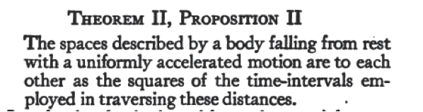
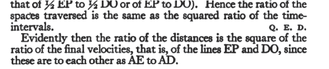
Basically, Galileo presented that not only was the acceleration down a ramp due to gravity constant, but that the velocity increased linearly with time. He presented that position increased with the square of the time, which is often referred to as the Law of Falling Bodies. The last point in this passage he presented is that velocity increased with the square of the distance down the ramp.
Building on what you have learned so far and what Galileo presented, we have what my physics teacher, Glenn Glazier, liked to call the Five Sacred Equations of Kinematics for constant acceleration. In these equations, v is velocity, x is position, t is time, and a is acceleration. Remember, Δ means change in.
1. ![]() or Δx = vavgΔt
or Δx = vavgΔt
2. ![]() or vf = vo + aΔt or Δv= aΔt
or vf = vo + aΔt or Δv= aΔt
3.![]()
4. Δx = vo Δt + ½ a Δt2
5. vf2=vo2 +2aΔx
The first two equations we have seen before. It is important to notice that the first equation uses average velocity, whereas the second equation uses the change between the original and final velocity. The connection between these is presented in the third equation which is simply the law of averages. The average velocity is the mean of the original and final velocity.
From these three basic definitions we can derive the next two equations using either geometry or algebra (or calculus).
Using algebra, we can derive equation #4.
Starting from equation #1
Δx = vavgΔt
We then substitute in the definition for average velocity from equation #3.
![]()
From here we subsitute in the final velocity arrived at in equation # 2
![]()
Next, we distribute the Δt term, and simplify by combining the vo terms.
![]()
We simplify the remaining two terms to arrive at
![]()
It is worthwhile to note what happens when the original velocity, vo, is zero. This equation simplifies even further to become
![]()
If we assume that the original position and time are zero, we can further reduce this to
![]()
Using geometry, we can examine the area under a curve of a velocity vs time graph for constant accelerating motion.
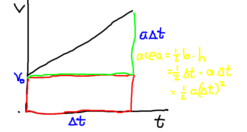
If we look at the area under the curve, we can break it into a rectangle and a triangle. The red rectangle is the contribution from the original velocity of the object. The displacement due to acceleration is represented by the green triangle. The triangle has a width of Δt, and a height of aΔt which we know from equation #2. The ½ term comes from the formula for the area of a triangle.
We can also use calculus to derive this equation by integrating twice the acceleration with respect to time.
The fifth sacred equation can be derived by similar substitutions and will be left as a homework problem.
Now let us look at some example problems: Numerical problem solving.
Example 1
By legend, Galileo dropped a ball from the Tower of Pisa. If the tower has a height of 55.9 m, and neglecting air resistance, how much time would it take a lead ball to reach the ground?
Givens: a = g ≈ 10 m/s2
Δx = 55.9 m
Unknown: t = ???
The equation that connects these variables is the 4th sacred equation.
Δx = voΔt + ½ a Δt2
As mentioned before, since the initial velocity is zero, the equation simplifies.
Δx = voΔt + ½ a Δt2 = ½ a Δt2
As we want to isolate the variable for time, we cross multiply to move the ½ and the acceleration term to the other side.
![]()
Next we take the square root of both sides.
![]()
This results in an expression for time. Note that I inserted some extra sets of parenthesis that you might not find necessary.
![]()
When plugging in the numbers it is fairly straightforward what we call plug and chug. However, you need to be careful with the units. You may have guessed that the time would be measured in seconds. However, you should be able to cancel the actual units to arrive at seconds for time.
Example 2
A coyote falls off a cliff with a height of 25 meters. How fast is the coyote falling when it hits the ground? If the coyote problem
Given x = 25 m
a = g ≈ 10 m/s2
Unknown: v = ???
There is more than one way to go about solving this problem. One could use a combination or Sacred equations # 2 and #4. Or you could directly use equation #5.
Using vf2=vo2 + 2aΔx
This simplifies because the original velocity, vo, is zero.
If we take the square root of both sides of the equation
![]()
![]()
![]()
Note how you take the square root of the units to get m/s.
We will leave solving this problem with two equations for a homework problem.
Recap on graphing and slope and area under curves problems
By examining position, velocity, and acceleration graphs you should be able to draw them interchangeably.
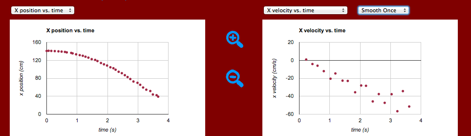
You saw yesterday in class that the graph of an object accelerating down a hill looks like this:
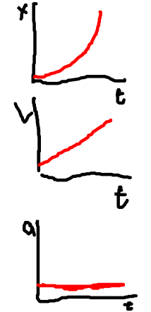
We are using the image analysis software in this example. This is an example with a ball rolling down the hill. One thing to note is that an acceleration graph does not tell you what the actual velocity is, just how it is changing. Likewise, the velocity graph does not give you the actual position of the object, just how it is changing. By clicking on the ball and hitting the track button, you will see a position and velocity graph generated.

Here you can see the results of graphing the motion. The position graph is a parabola and the velocity graph is linear.