Night 5 Reading:Acceleration
Acceleration can be defined as a change in velocity over a period of time. Usually, we think of this as a change in speed. Remember, velocity is a vector with both a magnitude and a direction. So there are two ways to change the velocity of an object. We can change either the speed or the direction of that speed (or both at the same time!)
Like velocity, acceleration is a vector with a magnitude and a direction. If the direction of the velocity is not changing, then we can express the acceleration as the rate of change of the speed,
![]()
Where a is acceleration, v is velocity, and t is time.
Since velocity is the rate of change of position, we could also think of acceleration as the rate of change of the rate of change. Acceleration is how much we speed up (or down) in a given second.
If you were watching a car advertisement, they might tell you that a car can go from 0 to 60 miles per hour in 6 seconds. Thus the units for acceleration might be given as miles/hour/second.  Although useful for cars and aircraft, in science we usually express velocity in terms of meters/second. Thus the units for acceleration would be meters/second/second. We can actually simplify this to meters/seconds squared.
![]()
Example 1:
 Suppose an airplane accelerates from 0 m/s to 50 m/s in 20 seconds. What would the acceleration of the plane be?
Δv = 50.0 m/s
Δt = 20. s
a = ?
![]()
In this case, you might note that the time only has two significant figures due to the location of the decimal point (although velocity has three).
EXAMPLE 2:
If a robot accelerates from rest at a rate of 2 , how fast is the robot moving after 4 seconds?
a = 2![]()
t = 4 s
Δv = ?
Using ![]() , we do algebra to isolate the velocity term.
, we do algebra to isolate the velocity term.
![]()
Notice how in the units, one factor of time (seconds) cancels out, leaving m/s as the units.
Constant Acceleration: When the acceleration is constant we can easily use the above equation to determine the change in velocity. If the acceleration is changing, we would have to use slightly more complex methods to find the change in velocity. Analytically, we could use calculus. Or, using a computer or a calculator we could use any of several approximation algorithms to find the change in velocity, similar to finding the change in position. In the case for a non-constant acceleration, we could even calculate the rate of change of the acceleration, which is called the jerk, as when you sharply tug or jerk a rope.
Circular Motion acceleration. The equation for acceleration for a circular path in the simplest case for non-linear acceleration. This is called an acceleration in a centripetal direction, or centripetal acceleration. We will return to this case when we study circular motion.
Most real-world accelerations are combinations of changes in speed and changes in direction. Another simple acceleration to analyze is when the object is vibrating back and forth. Often, the position of the object will follow a path similar to a sine wave. In this case, the acceleration is also a sine wave, a case we will explore when we get to vibratory motion.
Constant acceleration: graphs
When the acceleration is constant and positive then the a vs t graph will look like this.
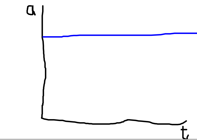
Since there is a constant acceleration, the velocity will increase as a linear function with respect to time and will appear like this. Of course, if one were to calculate the slope of the v vs t graph, one would find the acceleration.
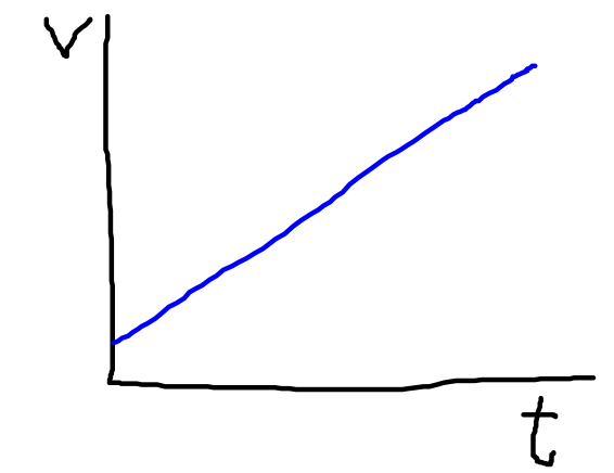
As we can see, the velocity is constantly increasing. What this means is that the distance traveled per second is constantly increasing. Likewise, the slope of our position vs time graph is constantly increasing, and will appear like the graph below. In this case the shape of the curve is a parabola, not a line. And the function which describes the graph is not linear but quadratic. Any quadratic term will have a squared term in it.

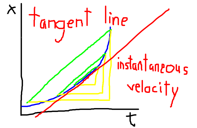
Recap of average velocity vs instantaneous velocity: Since the velocity is changing, the instantaneous velocity is not the same as the average velocity. We found the average velocity by finding the slope of the line created by two points. Since the velocity is changing, in this case we actually are finding the slope of a chord of this graph. As the chords become smaller we approach the limit for the instantaneous velocity.
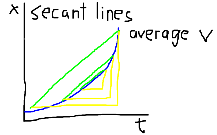
At the limit, we no longer have a chord of a finite length. Instead, we take a line which is tangent to the curve, and find the slope of this tangent line.
We will save a presentation of the equations for position under constant acceleration for the next lesson.