The direction of the velocity is important, even in the case for one-dimensional motion. Galileo investigated the issue of relative velocities.
The question of how velocities are all relative was wonderfully demonstrated in a video from the 1950’s by Dr. Hume for PSSC Physics called Frames of Reference.
Think of what happens when you step on a moving sidewalk at the airport. In the frame of reference of the moving sidewalk, you are moving at a casual pace. When you walk with the sidewalk, your velocity in the frame of reference of the ground is actually faster. If you were to foolishly walk against the sidewalk, your velocity in the ground’s frame of reference would actually be slow.
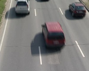
Another example If two cars are driving in the same direction, their relative velocities are the difference of the magnitude of their speeds. Consider when you are driving on the highway. You might be driving at 50 mph, when you are passed by a car driving at 55 mph. However it seems that they are passing you very slowly. Contra-wise, If two cars are driving in opposite directions from each other, their relative velocities are the sum of the magnitude of their velocities. 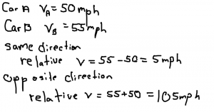
Another interesting problem you will explore in the homework has to do with finding average speeds. When you first learned about averages, you probably added two numbers together and divided the result by two. However, if you are working with a weighted average then you cannot use this simple trick by plugging in numbers.
Constant velocity: Position vs Time graph:
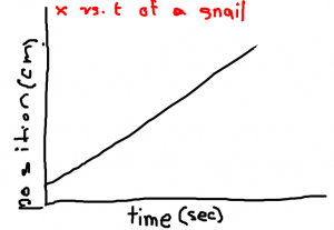
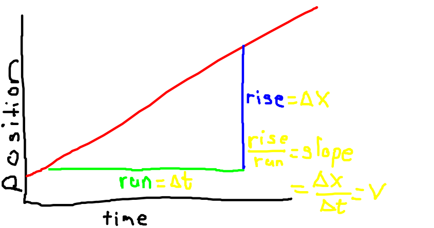
If we make a graph of position vs time and our object is moving at a constant velocity, the graph will form a straight line. We generally put position on the y-axis, and time on the x-axis. We call this a linear graph. The slope of this line will be the average velocity of our object. If the graph is flat or horizontal, then the object is not moving, the slope is zero, and the velocity is zero. It is important that when you have a graph, there is a title, axes labels, and units.
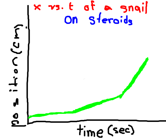
The faster the object goes, the greater the slope of the graph. In the following graph, you can see an object which is incrementally speeding up. Slow, fast, and faster.
Best fit line:
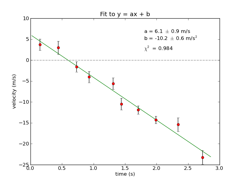
This is particularly useful for when there is a lot of noise in our data. In middle school, you may have learned to draw a best fit line by hand using a ruler. Computers calculate the best fit line using an algorithm called the Least Squares Fit. The computer calculates the error at every point, and tries to minimize the square of that error.
We can calculate the slope of the following graph. From middle school math, you may remember that you find the slope by taking the rise over the run.
Whenever you have a graph, you can always analyze the graph. It is not enough to merely say the graph goes up! The slope of the graph provides you with information, such as the velocity.
For a position vs. time graph, the
slope = rise/run = Δx/Δt
which of course we know as velocity! We should point out that if the slope is positive, then the velocity is positive. If the slope is negative and the graph goes down, then the velocity is negative relative to a reference point.
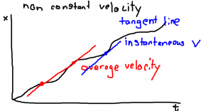
This could be particularly useful if the velocity of the graph is not constant. By finding the slope of a line tangent to the graph, we can actually find the instantaneous velocity at any given point in time. We will explore this in depth when we introduce acceleration.
Constant velocity: Velocity vs Time graph:
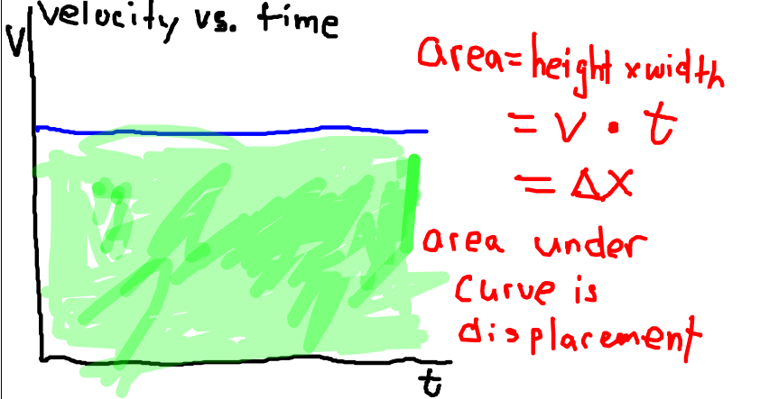
If the velocity of an object is constant, our v vs t graph is rather simple. It would look like this.
Note the units for both velocity and time. In this case, the slope of our graph is zero. What this means is the velocity is not changing. It is not accelerating.
But there is still a lot of information we can glean from this graph. In this case we will examine the “area under the curve.” The shape of the area under this graph is a simple rectangle.
The area of this rectangle is easy to calculate. In this case, the area is the base x height of the graph.
Area = velocity x time
If we review our kinematic equation, we quickly realize that the area under the curve is actually the displacement.
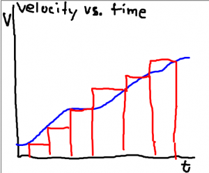
This general rule that the area under the curve of a velocity vs time graph is the displacement holds even when the velocity is not constant. In those cases, the area is not a simple rectangle and can be difficult to calculate exactly. But often, one can approximate with great accuracy this area for a non-constant velocity.
